Chipmunq: A Fault-Tolerant Compiler for Chiplet Quantum Architectures

A self-contained walkthrough of arXiv:2603.16389

Author

Based on Wegmann, Świerkowska, Giortamis & Bhatotia (2026)

Introduction

Building a reliable quantum computer out of a single chip is already extraordinarily hard. Now imagine you need several chips, wired together with connections that are ten to a hundred times noisier than the links inside each chip. Every quantum compiler ever built assumes, more or less, that the hardware is one contiguous slab of qubits. The moment you break that assumption, three things go wrong at once: compilation times explode, the careful geometric structure that error correction depends on gets shredded, and noisy inter-chip links quietly destroy the very fault tolerance you were counting on. The authors of this paper call it a “compilation wall” – and then proceed to knock it down.

This paper (arXiv: 2603.16389) was published in March 2026 by researchers at the Technical University of Munich (TUM).

Two trends on a collision course

To understand why this wall exists, we need to see two engineering trends that are individually promising but jointly create a headache.

Trend 1: Quantum Error Correction demands massive, structured qubit arrays. Fault-tolerant quantum computing encodes each logical qubit across many physical qubits arranged in a precise geometric layout called a patch – typically a square grid in the surface code. A single logical CNOT via lattice surgery might require three or more such patches, each containing $d^2$ physical qubits for code distance $d$. At the practically relevant distance $d \approx 27$, that is over 700 physical qubits per patch and thousands per logical operation. The geometry is not optional: break the patch shape and you break the error correction.

Trend 2: Chiplet architectures split the hardware across multiple dies. No single chip can reliably manufacture all those qubits. Fabrication yields drop, control wiring becomes unmanageable, and cryogenic cooling hits its limits. The solution, borrowed from classical computing, is to go modular: build smaller chips (chiplets) and connect them via microwave couplers or bump bonds. This buys you scalability – but the inter-chiplet links are sparse, slow, and 10–100x noisier than on-chip connections. Consider a concrete example: 4 chiplets of 1,000 qubits each, connected by roughly 20 inter-chip couplers per boundary. Each coupler has a two-qubit gate error rate of about 1%, compared to 0.1% within a chip — a 10x noise penalty for every operation that crosses a chip boundary.

Put these two trends together and you face a compilation problem that no existing tool solves well. Qubit-level compilers like LightSABRE time out on circuits with thousands of qubits. QEC-aware tools like QECC-Synth respect patch geometry but cannot scale past modest code distances. Chiplet-specific compilers like MECH operate at the qubit level and pile on gate overhead. None of them treat the noisy inter-chip links as a first-class concern.

TU Munich and the modular quantum computing movement

Chipmunq comes from the Chair of Design Automation at the Technical University of Munich, a group with a long track record in quantum compilation and architecture-aware design tools. They are not alone in betting on chiplets: IBM has pursued modular quantum processors since its Heron roadmap, connecting separate quantum chips via classical and quantum links. Intel has leveraged its semiconductor packaging expertise to fabricate multi-die quantum processors using flip-chip bonding. Google and Rigetti have explored similar paths. The shared conviction is that monolithic scaling will hit a ceiling, and modular architectures are the way through it. What has been missing – until now – is a compiler that actually understands the implications of that modularity for fault-tolerant circuits.

What Chipmunq does

The key insight behind Chipmunq is deceptively simple: work at the patch level, not the qubit level. A fault-tolerant circuit with thousands of physical qubits might only contain a few tens of logical patches. By detecting those patches first and treating them as indivisible units, the compiler reduces a seemingly intractable problem to a manageable one.

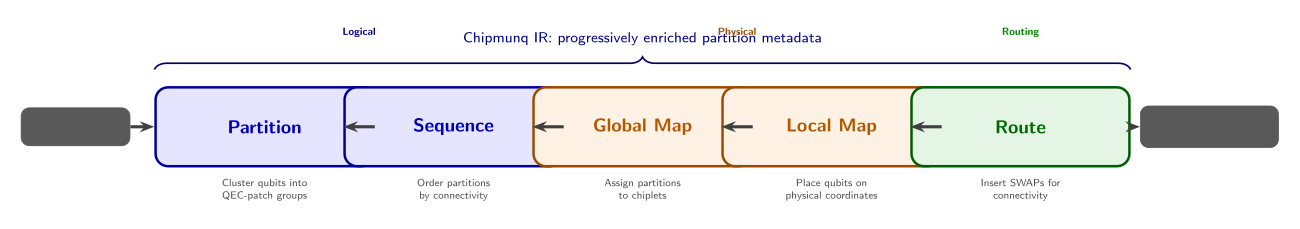
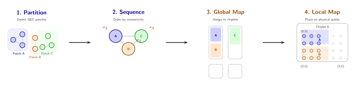
Concretely, Chipmunq is a five-stage pipeline:

Partition – Community detection algorithms identify QEC patches in the circuit’s dependency graph and group operations accordingly.
Sequence – A dependency-aware ordering determines which patches get placed first, prioritizing the most heavily connected ones.
Global map – Partitions are assigned to physical chiplets via 2D bin-packing that respects capacity, connectivity, and defective qubits.
Local map – Within each chiplet, logical qubits are placed onto physical qubits while preserving patch geometry.
Route – A cost-aware router inserts the minimal SWAP operations needed for nearest-neighbor connectivity, explicitly penalizing noisy inter-chiplet links.

An intermediate representation (the Chipmunq IR) threads through all five stages, carrying an immutable logical dependency graph alongside progressively enriched hardware-binding metadata. Each stage adds information without disturbing the logical structure that earlier stages established.

Results at a glance

Let’s preview what this buys us. Compared to LightSABRE (the state-of-the-art general-purpose baseline from IBM’s Qiskit), Chipmunq achieves:

13.5x faster compilation on average, with up to 70x speedup at higher circuit complexity.
86.4% reduction in circuit depth and 91.4% fewer SWAP gates, because patch-aware placement avoids the avalanche of routing corrections that qubit-level compilers trigger.
Up to 100x better logical error rates in heterogeneous noise environments, by steering critical syndrome measurements away from low-fidelity inter-chiplet links.

Remark. Remark. Notice the asymmetry in these results: the depth and SWAP improvements are large but incremental refinements of existing compiler capabilities. The logical error rate improvement is qualitatively different – it is the difference between error correction that works and error correction that fails. This is where chiplet-awareness matters most.

Roadmap

In the rest of this document, we will build up the full picture step by step. We begin with the background needed to follow the paper: surface codes, lattice surgery, and chiplet hardware models (Section 2). Next, we walk through the motivation, showing quantitatively why existing compilers fail (Section 3). We then unpack each stage of the Chipmunq pipeline in detail (Section 4 and Section 5), followed by a guided tour of the evaluation results (Section 6). Finally, we discuss limitations and open questions (Section 7).

Background

Before we get into Chipmunq’s design, let’s lay the groundwork. We need three pieces: what fault-tolerant quantum computing demands at the physical level, why chiplet architectures are the likely path to scaling, and what a quantum compiler actually has to do. If you’re already comfortable with surface codes and lattice surgery, feel free to skim ahead to the chiplet section.

Quantum Error Correction and Surface Codes

Physical qubits are noisy. Every gate we apply, every microsecond a qubit sits idle, errors creep in — bit-flips, phase-flips, leakage to unwanted energy levels. A single physical qubit today has an error rate somewhere around $10^{-3}$ per operation in the best cases. That sounds decent, but a useful quantum algorithm (say, breaking RSA-2048 or simulating a catalyst) requires billions of operations. At $10^{-3}$ error per gate, the computation is overwhelmed by noise long before it finishes.

The solution is quantum error correction (QEC): we encode one logical qubit into many physical qubits, spreading the information so that individual physical errors can be detected and corrected without destroying the encoded state. The idea is the quantum analogue of classical parity checks — we measure certain multi-qubit operators (called stabilizers) that reveal whether an error occurred and where, without collapsing the encoded quantum information.

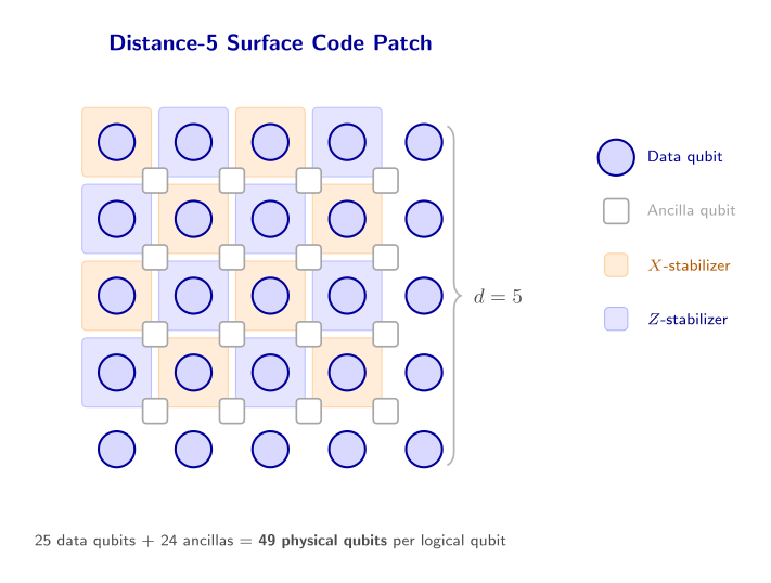
The surface code is the workhorse of fault-tolerant quantum computing. It arranges physical qubits on a 2D square grid, alternating between data qubits (which carry the encoded information) and ancilla qubits (which are measured repeatedly to extract error syndromes). Each ancilla measures a local parity check — either an $X$-type or $Z$-type stabilizer — involving its neighboring data qubits. The 2D nearest-neighbor layout is crucial: it matches the connectivity constraints of real hardware, where qubits can only interact with their immediate neighbors.

Code distance. The distance $d$ of a surface code is the minimum number of single-qubit errors needed to cause a logical error (one that goes undetected and corrupts the encoded information). A distance-$d$ surface code uses $\mathcal{O}(d^2)$ physical qubits and can correct up to $\lfloor(d-1)/2\rfloor$ errors per round of syndrome extraction. The logical error rate scales as $p_L \sim (p/p_\text{th})^{\lfloor d/2 \rfloor}$, where $p$ is the physical error rate and $p_\text{th} \approx 1\%$ is the threshold. Each increase in $d$ suppresses $p_L$ exponentially — provided we stay below threshold.

Seeing the numbers. With $d = 3$ we use $3^2 = 9$ data qubits (plus ancillas, so about 17 physical qubits total) and can correct $\lfloor(3-1)/2\rfloor = 1$ error per round. At physical error rate $p = 0.001$ and threshold $p_\text{th} \approx 0.01$, the logical error rate scales as $p_L \sim (0.001/0.01)^{\lfloor 3/2 \rfloor} = (0.1)^1 = 10\%$. Bump to $d = 5$ (25 data qubits, ~49 physical qubits): $p_L \sim (0.1)^2 = 1\%$. At $d = 7$: $p_L \sim (0.1)^3 = 0.1\%$. Each $+2$ in distance buys roughly an order of magnitude in logical error suppression — but at the cost of quadratically more physical qubits.

A distance-5 surface code patch. Data qubits (blue circles) sit on the vertices of a $5 \times 5$ grid, while ancilla qubits (gray squares) occupy the faces, each measuring either an $X$-stabilizer (orange) or $Z$-stabilizer (blue) involving its neighboring data qubits.

A surface-code patch is the physical realization of one logical qubit: a $d \times d$ region of qubits with its own set of stabilizer measurements. To perform a useful computation, we need to execute logical gates between patches.

A distance-$d$ surface code patch contains $d^2$ data qubits and $(d-1)^2 + d^2 - 1$ ancilla qubits — roughly $2d^2$ physical qubits total.

For instance, a distance-5 surface code patch is a $5 \times 5$ grid of data qubits (25 total) plus 24 ancilla qubits for syndrome extraction, giving 49 physical qubits for one logical qubit. A logical CNOT via lattice surgery needs 3 such patches (control, target, and ancilla), totaling $3 \times 49 = 147$ physical qubits minimum. At distance 15, that becomes $3 \times 421 \approx 1{,}263$ physical qubits for a single logical CNOT.

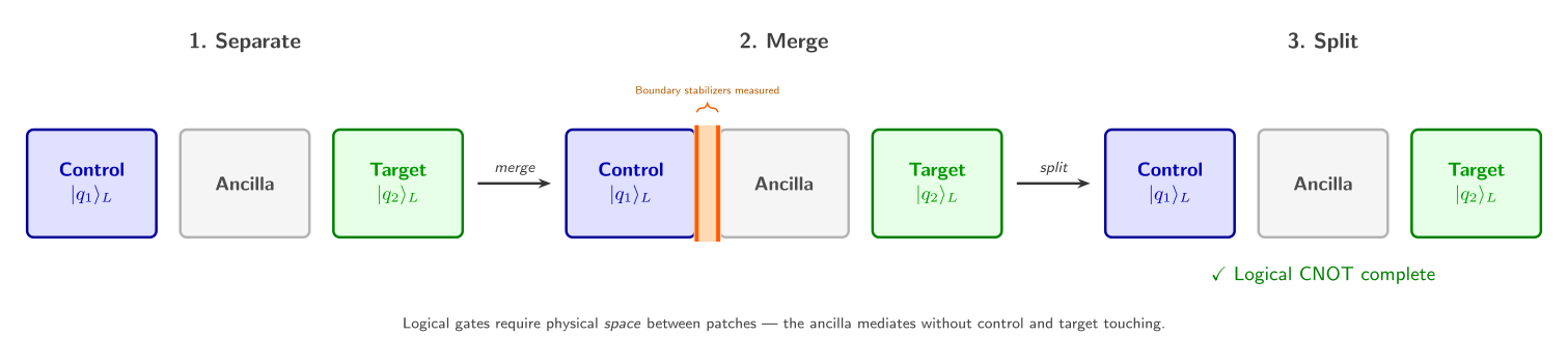
This is where lattice surgery comes in. Rather than physically moving qubits, we perform logical multi-qubit gates by merging adjacent patches (measuring stabilizers across their shared boundary) and then splitting them apart. A logical CNOT, for instance, requires three patches: two data patches (the control and target qubits) plus one ancilla patch that mediates the interaction. The merge-and-split sequence effectively performs a joint logical measurement, implementing the gate. Notice that this means every logical operation needs physical space between patches — a constraint that profoundly shapes how we lay out and route computations.

Lattice surgery in three steps. (1) Three surface-code patches — control, ancilla, and target — sit side by side with gaps between them. (2) Merge: stabilizers are measured across the shared boundary of the control and ancilla patches (highlighted region), entangling them. (3) Split: the boundary stabilizers are turned off and the patches separate, completing the logical CNOT. The ancilla patch mediates the interaction without the control and target ever touching directly.

Chiplet Architectures

Building a single monolithic quantum chip with millions of qubits is extraordinarily difficult. As chip size grows, fabrication yield drops (a single defect can ruin the whole device), wiring complexity explodes, and frequency crowding degrades performance. At some point, we hit a wall.

Chiplet architecture. A chiplet architecture partitions the quantum processor into multiple smaller chips (chiplets), each containing a manageable number of qubits ($\sim$hundreds to low thousands). Chiplets are connected via inter-chip links — physical connections (microwave resonators, photonic links, or direct coupler lines) that enable entangling operations between qubits on different chiplets.

The idea borrows directly from classical computing, where multi-die packages are now standard (think AMD’s Ryzen or Intel’s Ponte Vecchio). Each chiplet can be fabricated and tested independently, dramatically improving yield. A 1000-qubit monolithic chip with 99% per-qubit yield would have only a $$0.004% chance of being defect-free; four 250-qubit chiplets each have a $$8%$ chance, and we only need all four to work.

A concrete picture. Imagine four chiplets arranged in a $2 \times 2$ grid. Each chiplet holds 100 physical qubits arranged in a $10 \times 10$ lattice with full nearest-neighbor connectivity within the chip. But the inter-chiplet boundary has only 8 link qubits connecting each pair of adjacent chiplets. These links are 10–100$\times$ noisier than on-chip gates (error rates of $1$–$10\%$ vs. $0.1\%$) and orders of magnitude sparser (8 links vs. 100 possible boundary positions). Any operation that crosses a chiplet boundary pays a heavy penalty.

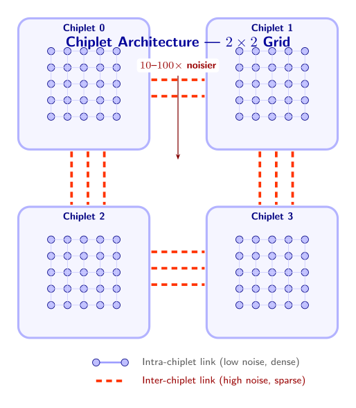
A 2x2 chiplet architecture. Each chiplet (rounded box) contains a dense grid of qubits with high-fidelity nearest-neighbor connections. Inter-chiplet links (dashed red) are sparse and $10\text{--}100\times$ noisier, creating the asymmetry that drives the need for chiplet-aware compilation.

This asymmetry — dense, high-quality connections within a chiplet and sparse, noisy connections between chiplets — is the defining challenge. A compiler that ignores chiplet boundaries will route operations across noisy links whenever it is convenient, producing circuits that fail in practice. We need a compiler that is chiplet-aware.

The Quantum Compilation Pipeline

A quantum compiler translates a logical quantum algorithm — expressed as a circuit of gates on abstract qubits — into physical instructions that a specific piece of hardware can execute. This is conceptually similar to a classical compiler, but the constraints are far more brutal.

The standard compilation pipeline has several stages:

Synthesis: decompose high-level gates into the hardware’s native gate set (e.g., express a Toffoli gate as a sequence of CNOTs and single-qubit rotations).
Mapping (also called placement): assign each logical qubit to a specific physical qubit on the device.
Routing: when a gate requires two qubits that are not physically adjacent, insert SWAP gates to shuffle qubits along the connectivity graph until they become neighbors.
Scheduling: determine the time ordering of operations, parallelizing where possible while respecting hardware constraints.

A SWAP gate exchanges the states of two adjacent qubits. It costs 3 CNOT gates, so every SWAP we insert adds noise. Minimizing the number of inserted SWAPs is a central goal of any router.

Mapping and routing are where the real difficulty lies. Mapping is equivalent to subgraph isomorphism and is NP-hard; routing (minimizing inserted SWAPs) is similarly NP-hard. In practice, we rely on heuristics — greedy algorithms, simulated annealing, reinforcement learning — that find good-enough solutions in reasonable time.

Let’s see this concretely: a single SWAP gate decomposes into 3 CNOT gates. If a router inserts 1,000 SWAPs to route a distance-7 circuit, that is 3,000 extra CNOTs, each with roughly 0.1% error rate. The probability of no error across those extra gates is $(1 - 0.001)^{3000} \approx 5\%$ — meaning the inserted routing overhead alone introduces an error with 95% probability. The noise from routing can easily drown out the error correction the circuit was designed to perform.

Remark. Why this is harder for fault-tolerant chiplet systems. At the fault-tolerant level, we are no longer routing individual physical qubits — we are routing patches made of $\mathcal{O}(d^2)$ qubits each. A 100-logical-qubit circuit at distance $d=17$ involves over 50,000 physical qubits. The circuit depth grows by a factor of $d$ as well, since each logical gate requires $d$ rounds of syndrome extraction. On top of this, every patch must maintain its 2D geometry and stabilizer measurements throughout the computation. And on a chiplet system, every inter-chiplet crossing must be budgeted carefully: we need to either route patches so they avoid boundaries entirely, or explicitly allocate noisy link operations and compensate with additional error correction. This is the problem Chipmunq was built to solve.

The Compilation Wall

Fault-tolerant quantum computing on chiplet hardware sounds like a clean division of labor: QEC handles the noise, chiplets handle the scale. In practice, the two collide at the compiler. The compiler must take a fault-tolerant circuit — already bloated by error-correction overhead — and map it onto a modular processor whose inter-chip links are sparse and noisy. This section walks through three concrete ways that existing compilers break down when confronted with this task, building toward the problem statement that Chipmunq addresses.

Challenge 1: The Scalability Crisis

Start with the raw numbers. A rotated surface code patch at distance $d$ uses roughly $d^2 + (d-1)^2$ physical data and syndrome qubits. At $d = 15$, that is about 421 physical qubits for a single logical qubit — a patch that encodes one $\ket{0}_L$. A logical CNOT via lattice surgery requires three such patches (two data patches plus an ancilla patch for the merge/split), so one logical CNOT at $d = 15$ involves approximately 1,350 physical qubits and thousands of physical gates. Push to $d = 27$ — the distance Google estimates is needed for practical fault-tolerant operation — and a single logical CNOT balloons to over 4,000 physical qubits.

Google’s 2025 surface-code experiments project that practical fault tolerance will require code distances on the order of $d \approx 27$.

This explosion in circuit size crushes compilers that were designed for the NISQ era. The authors benchmark three representative tools on surface-code memory circuits of increasing distance:

QECC-Synth (QEC-aware): produces high-quality, structure-preserving mappings but hits a 1,000-second timeout at $d = 11$. It simply cannot finish the job at the distances that matter.
MECH (chiplet-aware): scales more gracefully with approximately linear runtime growth, but still becomes impractically slow at large distances.
LightSABRE (general-purpose, part of Qiskit): maintains sub-second compilation across all evaluated distances, showing no clear scaling trend.

Compilation runtime, gate overhead, and inter-chiplet utilization for a single surface code patch, comparing LightSABRE, MECH, and QECC-Synth across increasing code distances.

So the only compiler that stays fast enough is LightSABRE — a general-purpose tool with no knowledge of QEC structure or chiplet constraints. That brings us to the next problem.

For instance, a single logical CNOT at $d = 15$ produces roughly 1,350 physical qubits and $$10,000 physical gates. QECC-Synth, which explores a combinatorial space to preserve patch geometry, sees a routing problem of size $1{,}350^2 \approx 1.8 \times 10^6$ qubit pairs — and times out well before finishing. LightSABRE finishes in under a second because its heuristic is lightweight, but it treats all 1,350 qubits as independent entities, oblivious to the fact that they form three structured patches.

Remark. Remark. The scalability wall is not an implementation bug — it reflects the NP-hardness of qubit routing. QECC-Synth explores a large solution space to preserve patch geometry; the cost is exponential blowup. LightSABRE uses lightweight heuristics that sidestep the explosion, but as we will see, it pays a steep price in solution quality.

Challenge 2: Patch Fragmentation

A surface code patch is not just a bag of qubits. It is a carefully structured 2D lattice: data qubits sit at specific positions, $X$- and $Z$-stabilizer ancillas occupy interleaved sites, and the boundary conditions (rough vs. smooth edges) determine how logical operators are defined. Disturb this geometry — move a data qubit away from its stabilizer neighbors — and the error-correction machinery fails. The patch stops being a valid code.

Patch-preserving compilation. A compiler is patch-preserving if, after mapping and routing, every QEC patch retains its original geometric structure: the relative positions of data qubits, syndrome qubits, and their connectivity are unchanged. No SWAP operations break the patch interior.

General-purpose compilers like LightSABRE have no concept of patches. They see a circuit of physical qubits and two-qubit gates, and they insert SWAP gates to bring interacting qubits into nearest-neighbor contact on the hardware connectivity graph. This process freely shuffles qubits around the chip — exactly what destroys patch structure.

Mosaic analogy. Imagine you have carefully tiled a mosaic — each colored tile is in a precise position to form the image. Now someone reaches in and swaps a few tiles to make room for a new piece. The individual tiles are fine, but the pattern is destroyed. That is what SWAP insertion does to a surface code patch: the physical qubits still exist, but they are no longer arranged in the lattice that the decoder expects.

The paper quantifies this with a clean experiment. The authors compile a single surface-code patch onto a monolithic grid whose geometry exactly matches the patch layout. An ideal compiler should introduce zero additional two-qubit gates — the patch fits the hardware perfectly. The results tell a stark story:

QECC-Synth maintains zero overhead across all distances. It knows about patch structure and preserves it.
LightSABRE begins violating patch integrity at $d = 9$ and introduces rapidly increasing two-qubit gate overhead beyond that point.
MECH introduces nearly linear gate overhead across all evaluated distances.

Two-qubit gate overhead introduced by each compiler when mapping QEC patches onto a monolithic backend. An ideal, patch-preserving compiler achieves zero overhead.

The overhead is not merely wasteful — it is actively harmful. Every inserted SWAP is three additional CNOT gates, each of which injects noise into the middle of the error-correction cycle. At high enough overhead, the added noise overwhelms the code’s ability to correct errors, and the logical error rate starts increasing with code distance instead of decreasing. The patch is formally intact on the hardware, but functionally broken.

Challenge 3: Interconnect Heterogeneity

Suppose a compiler could partition and place patches correctly, keeping each patch intact within a single chiplet. There is still a third trap: not all connections are created equal.

In a chiplet architecture, intra-chiplet qubit couplings are fast, low-noise, and dense. Inter-chiplet links — whether microwave couplers, bump bonds, or photonic interconnects — are typically 10–100x noisier than on-chip gates. A compiler that treats all connections as equivalent will happily route critical syndrome-extraction circuits over these noisy links, unaware that it is undermining the very error correction those circuits implement.

Inter-chiplet error rates can be $10\text{--}100\times$ higher than intra-chiplet rates, a heterogeneity that no general-purpose compiler currently accounts for.

The authors test this by compiling patches onto a chiplet backend where each chiplet is sized to comfortably fit one patch. In this configuration, a smart compiler should keep each patch entirely within a single chiplet and avoid inter-chiplet links altogether. The results show that none of the existing compilers achieve this:

LightSABRE and MECH both exhibit approximately linear growth in the number of two-qubit gates executed over inter-chiplet connections as circuit size increases.
QECC-Synth achieves lower inter-chiplet utilization by exploiting mechanisms designed for sparse architectures, but still introduces a non-negligible and growing number of inter-chiplet operations.

Number of two-qubit gates executed over inter-chiplet connections. All three compilers unnecessarily route operations across noisy inter-chiplet links.

The consequence is direct: syndrome measurements that should run on high-fidelity local connections instead traverse noisy inter-chiplet links. This injects correlated errors that the surface code decoder is not designed to handle at that rate. The logical error rate climbs above the correction threshold, and increasing the code distance no longer helps — you are throwing more resources at a problem the compiler created.

For instance, consider a distance-7 patch whose syndrome extraction circuit runs 7 rounds per logical gate. If a compiler routes just 4 of the patch’s 24 stabilizer measurements across an inter-chiplet link with error rate $p = 0.01$ (versus $p = 0.001$ on-chip), those 4 stabilizers contribute $4 \times 7 \times 0.01 = 0.28$ expected errors per logical gate — compared to $4 \times 7 \times 0.001 = 0.028$ if they stayed on-chip. That 10x noise injection on a small fraction of stabilizers can push the effective error rate above the code’s correction threshold, causing the logical error rate to increase with distance instead of decrease.

Remark. Remark. The heterogeneity problem is subtle because it is invisible at the circuit level. The compiled circuit may have the correct gate count and depth, but because some of those gates execute over links with 10x higher error rates, the effective noise budget is blown. Architecture-awareness is not an optimization — it is a correctness requirement.

The Problem Statement

These three challenges — scalability, patch fragmentation, and interconnect heterogeneity — are not independent. They reinforce each other. The only compiler that scales (LightSABRE) fragments patches and ignores link quality. The only compiler that preserves patches (QECC-Synth) cannot scale. No existing tool accounts for inter-chiplet noise heterogeneity. This brings us to the central question of the paper:

Problem statement. How can fault-tolerant quantum circuits be mapped and routed onto chiplet-based architectures in a scalable, QEC patch-preserving, and architecture-aware manner?

Chipmunq’s answer — a five-stage pipeline that reasons about patches rather than individual qubits — is the subject of the next sections.

Chipmunq Architecture

Now that we understand the problem — compiling fault-tolerant circuits onto chiplet hardware while preserving QEC patch structure — let’s see how Chipmunq actually works. The key idea is a five-stage pipeline where each stage adds information to an intermediate representation without destroying what the previous stages computed. Think of an assembly line where each station adds a component, and nothing gets disassembled along the way.

The Five-Stage Pipeline

The figure below shows the full pipeline at a glance.

The Chipmunq five-stage pipeline. Logical stages (blue) discover and order QEC patches; physical stages (orange) bind them to hardware; the router (green) inserts SWAPs. The Chipmunq IR is progressively enriched at each stage.

Each stage solves one sub-problem, and critically, the stages are compositional: the partitioner knows nothing about chiplets, the sequencer knows nothing about physical qubit coordinates, and the router receives a fully mapped circuit. This clean separation is what makes Chipmunq modular — you can swap out the partitioner without touching the router, or target a different backend by changing only the global and local mappers.

Remark. Why five stages, not three? Existing compilers like LightSABRE or SABRE fold mapping and routing into a single pass. Chipmunq deliberately separates global mapping (which chiplet?) from local mapping (which physical qubits on that chiplet?) and both from routing (which SWAPs to insert?). This decomposition keeps each sub-problem tractable and allows each stage to exploit structure that a monolithic pass would miss — for instance, the global mapper can reason about chiplet adjacency without worrying about individual qubit coordinates.

The Chipmunq Intermediate Representation

The glue that holds the five stages together is the Chipmunq IR — a data structure that accumulates hardware-binding information as it passes through the pipeline. This is the central software design contribution of the paper.

Think of it as a passport that accumulates stamps at each border crossing. The passport itself (the circuit DAG) never changes — but each stage stamps it with new metadata (partitions, ordering, chiplet assignments, physical coordinates) until, at the end, the passport carries all the information needed for hardware execution.

Chipmunq IR. The IR $\mathcal{I}$ is a 2-tuple $(G, \Pi)$:

$G = (V, E)$ is a Directed Acyclic Graph representing the quantum circuit. $V$ is the set of quantum operations (gates), $E$ encodes qubit dependencies. $G$ is immutable — no stage modifies it until the final routing pass produces the output DAG.
$\Pi = \{\pi_1, \pi_2, \ldots, \pi_n\}$ is the partition registry, a set of stateful partition objects that get progressively enriched with hardware-binding metadata.

Each partition $\pi_i \in \Pi$ is defined as: \[ \pi_i = \langle Q_i, \sigma_i, \alpha_i, \phi_i \rangle \]

where:

Field	Set by	Meaning
$Q_i \subset Q_\text{virt}$	Partitioner	Which virtual qubits belong to this partition
$\sigma_i \in \mathbb{Z}_{\geq 0}$	Sequencer	Execution order (position in global schedule)
$\alpha_i$	Global mapper	Chiplet assignment (which chiplet this partition lives on)
$\phi_i : Q_i \to P(x,y)$	Local mapper	Physical qubit coordinates within chiplet $\alpha_i$

For instance, consider a circuit with 3 logical qubits performing one CNOT. The partitioner might produce 4 partitions (3 data patches + 1 ancilla). Initially each $\pi_i$ only has $Q_i$ (its qubit list). After sequencing, $\pi_1$ gets $\sigma_1 = 0$ (placed first, since it is most connected), $\pi_2$ gets $\sigma_2 = 1$, and so on. After global mapping, $\pi_1.\alpha = \text{chiplet}_0$ and $\pi_2.\alpha = \text{chiplet}_0$ (same chip, because they interact heavily). After local mapping, $\pi_1.\phi$ maps its 49 virtual qubits to physical coordinates $(0,0)$ through $(6,6)$ on chiplet 0.

The compilation process is a chain of enrichment functions, each strictly increasing the information density of $\Pi$:

\[ G \xrightarrow{f_\text{part}} \Pi_{\{Q\}} \xrightarrow{f_\text{seq}} \Pi_{\{Q,\sigma\}} \xrightarrow{f_\text{gmap}} \Pi_{\{Q,\sigma,\alpha\}} \xrightarrow{f_\text{lmap}} \Pi_{\{Q,\sigma,\alpha,\phi\}} \xrightarrow{f_\text{route}} G_\text{final} \]

The subscripts on $\Pi$ indicate which fields have been filled in. After partitioning, each $\pi_i$ only has its qubit set $Q_i$. After sequencing, it also has an ordering $\sigma_i$. And so on. The unidirectional flow means that no stage ever needs to undo or revise work done by a previous stage.

Think of filling out a shipping label: first you write WHAT is in the package (partitioning fills in $Q_i$ — which qubits belong together), then WHEN it ships (sequencing fills in $\sigma_i$ — the execution order), then WHICH warehouse (global mapping fills in $\alpha_i$ — the chiplet assignment), then the EXACT shelf location (local mapping fills in $\phi_i$ — the physical qubit coordinates). Each line on the label depends on the ones above it, and once written, it is never erased.

The IR design is inspired by classical compiler IRs like LLVM’s, where passes progressively lower the representation from high-level to machine-specific. The key difference: in Chipmunq, the original circuit DAG stays intact throughout, and enrichment happens in the partition registry on the side.

Why an immutable DAG?

Keeping $G$ immutable until the final routing pass has a practical benefit: any stage can inspect the original circuit structure without worrying that a previous stage modified it. This makes debugging straightforward — you can compare the original DAG against the final routed DAG to see exactly which operations were inserted. It also enables the modular design goal: high-level FT compilation (lattice surgery) produces $G$ once, and Chipmunq can compile the same $G$ to different backends without re-running the expensive FT compilation step.

Workflow Walkthrough

The Chipmunq pipeline in action on a 3-logical-qubit circuit. (1) The partitioner detects QEC patches as communities in the qubit entanglement graph. (2) The sequencer orders partitions by connectivity. (3) The global mapper assigns partitions to chiplets via bin-packing. (4) The local mapper places virtual qubits onto physical coordinates within each chiplet.

Let’s trace through Chipmunq’s pipeline on the concrete example from the paper: a fault-tolerant circuit with three logical qubits and a single logical CNOT gate, targeting a backend with four chiplets.

Walkthrough of a 3-logical-qubit CNOT compiled onto a 4-chiplet backend. Each panel shows the IR state after one pipeline stage: partitioning identifies patches, sequencing orders them, global mapping assigns chiplets, and local mapping places physical qubits.

Input. The FT circuit encodes the CNOT via lattice surgery, which requires three surface-code patches (one for control, one for target, one ancilla patch mediating the interaction). After synthesis, this produces a circuit acting on many physical qubits with dense local interactions within each patch and sparse interactions between patches.

Step 1 — Partitioning. The partitioner analyzes the circuit DAG and identifies communities of densely interacting qubits. It detects four natural clusters — corresponding to the three logical patches plus the ancilla region — and splits the circuit into four partitions. Each partition $\pi_i$ now has its qubit set $Q_i$ filled in: “these virtual qubits belong together.”

Step 2 — Sequencing. The sequencer builds a dependency graph over the four partitions (which partitions need to interact?) and performs a BFS traversal. The most highly connected partition (say, Partition 1, which interacts with Partitions 2, 3, and 4) gets processed first. This ensures the global mapper has maximum flexibility when placing the most constrained partitions. Each $\pi_i$ now carries its ordering $\sigma_i$.

Step 3 — Global mapping. Given four chiplets in a $2 \times 2$ grid, the global mapper must assign partitions to chiplets. Following the sequence order, it places Partition 1 first. Partition 2 interacts heavily with Partition 1, so it goes on the same chiplet to avoid inter-chiplet communication. Partition 3 also interacts with Partition 1, so it goes on an adjacent chiplet (one that shares inter-chiplet links with Partition 1’s chiplet). Partition 4 has no strong connectivity constraints and goes on any remaining chiplet. Each $\pi_i$ now knows its chiplet assignment $\alpha_i$.

Step 4 — Local mapping. Within each chiplet, the local mapper translates the 2D bin-packing coordinates into actual physical qubit addresses. For Partition 4, the mapper notices defective qubits at two corners of the chiplet and adjusts the placement to avoid them while maintaining a square patch shape. Each $\pi_i$ now has its coordinate mapping $\phi_i$.

Step 5 — Routing. Finally, the router inspects every gate in the circuit. Gates within a single partition need no additional routing (the patch is already laid out with nearest-neighbor connectivity). For the interaction between Partitions 1 and 2 (same chiplet), the router inserts intra-chiplet SWAPs along a short path. For the interaction between Partitions 1 and 3 (different chiplets), the router must route through the sparse, noisy inter-chiplet links, carefully selecting which link to use based on fidelity and congestion. The output is $G_\text{final}$: a fully compiled DAG ready for hardware execution.

Remark. Notice the information flow. Each step consumes only the metadata produced by previous steps and adds its own. The partitioner never sees chiplet topology. The sequencer never sees physical qubit coordinates. This clean layering makes each stage independently testable and replaceable — a property that monolithic compilers like LightSABRE, which interleave mapping and routing in a single pass, cannot offer.

Design Deep Dive

The previous section gave us the 30,000-foot view. Now let’s open up each stage and see the algorithms inside. We will go in pipeline order: partition, sequence, map globally, map locally, route.

Partitioning

The partitioner’s job is to answer one question: which qubits belong together? In a fault-tolerant circuit, the answer is almost always “qubits within the same QEC patch.” But Chipmunq does not require the user to specify patches manually. Instead, it discovers them from the circuit structure.

Step 1: Build the qubit entanglement graph. From the input circuit DAG, Chipmunq constructs an undirected graph where each node is a virtual qubit and each edge connects two qubits that interact via a two-qubit gate. The weight of each edge reflects how many times those two qubits interact throughout the circuit. Qubits within the same surface-code patch interact dozens or hundreds of times (stabilizer measurements, data shuttling); qubits in different patches interact rarely (only during lattice surgery merge operations).

Step 2: Community detection. The entanglement graph is fed into the Girvan-Newman algorithm, a community detection method that iteratively removes the highest-betweenness edges to reveal natural clusters. The output is a list of communities and — crucially — the number of communities detected.

The Girvan-Newman algorithm runs in $\mathcal{O}(n^3)$ on a graph with $n$ nodes. For the qubit entanglement graphs typical in FT circuits (hundreds to low thousands of nodes), this is fast enough.

Chipmunq does not use the raw community assignments directly. Instead, it extracts the count of detected communities and uses that as the target partition count $k$ for the next step. This decoupling is deliberate: it lets the subsequent partitioner use algorithms that require a fixed $k$ as input, without being locked into the Girvan-Newman groupings.

Step 3: $k$-way partitioning. With $k$ in hand, Chipmunq models the partitioning as a $k$-way graph partitioning problem: split the qubit entanglement graph into $k$ groups of bounded size, minimizing the number of cut edges (interactions that cross partition boundaries). It delegates this to KaHyPar, a state-of-the-art hypergraph partitioner with near-logarithmic runtime.

Community detection: from Facebook to fault tolerance

The Girvan-Newman algorithm was originally developed for social network analysis — finding friend groups in networks like Facebook, or research clusters in citation graphs. The core insight is that edges between communities carry disproportionately high betweenness centrality (many shortest paths run through them), while edges within communities are redundant (there are many alternative paths). Removing high-betweenness edges peels the graph apart into its natural clusters. That the same technique works for QEC circuits is not a coincidence: a surface-code patch is a tightly connected community. Qubits within a patch interact every syndrome-extraction round; qubits across patches interact only during merge operations. The community structure is baked into the physics.

The result of partitioning is a set of partitions $\{\pi_1, \ldots, \pi_k\}$, each with its qubit set $Q_i$ filled in. One important detail: when the input circuit comes from a high-level FT compiler that already knows which qubits form which patch, the user can supply a predefined partition mapping (a dictionary from qubit to partition ID), skipping the detection step entirely. This is the common case for lattice-surgery circuits and avoids redundant computation.

Sequencing

With partitions defined, the sequencer must decide: in what order should we place them on the hardware? This matters because the global mapper is greedy — it processes partitions one at a time, and the first partition placed has the most freedom, while later partitions must work around earlier placements. Getting the order wrong means the most constrained partitions may end up in suboptimal positions.

The sequencer builds a partition dependency graph: nodes are partitions, edges connect partitions whose qubits interact (that is, partitions that will need to communicate at runtime). It then performs a BFS traversal starting from the most connected partition. The BFS discovery order becomes the mapping sequence.

BFS from the highest-degree node ensures that the most interconnected partition is placed first (maximum flexibility), and its immediate neighbors are placed next (while adjacent chiplet slots are still available).

The BFS also naturally groups partitions into connected components. If the input contains multiple independent circuits (say, two separate lattice-surgery operations that share no qubits), each component gets its own ordering. This enables concurrent compilation of multiple FT circuits onto a single backend — a feature enabled by the modular IR design.

Global Mapping

The global mapper takes the ordered list of partitions and assigns each to a chiplet. The mental model is bin packing: chiplets are bins with finite capacity, and partitions are rectangular items to be packed.

Chipmunq formulates this as a 2D bin-packing problem (2BP). Each chiplet is a rectangular bin whose dimensions correspond to the chiplet’s qubit grid. Each partition is a rectangular block whose dimensions are determined by the patch shape (for a distance-$d$ surface code, roughly $d \times d$). The goal is to pack all partitions into the available bins while minimizing the number of inter-bin (inter-chiplet) interactions.

Bin-packing in action. Imagine a $2 \times 2$ chiplet grid where each chiplet is a $15 \times 15$ qubit lattice (225 qubits). You have 4 surface-code patches: two at $d = 7$ ($7 \times 7 = 49$ qubits each) and two at $d = 5$ ($5 \times 5 = 25$ qubits each). Patch A ($7 \times 7$) goes into chiplet 0, centered. Patch B ($5 \times 5$) fits next to it on the same chiplet — the remaining $15 \times 8$ strip easily accommodates it — because A and B interact via lattice surgery. Patch C ($7 \times 7$) must go on chiplet 1 (adjacent to chiplet 0, since C interacts with A). Patch D ($5 \times 5$) has a defective $3 \times 3$ corner on chiplet 2, so the packer shifts D away from the damage, placing it in the clean region. Total: 4 patches across 3 chiplets, with inter-chiplet links only where unavoidable.

Two placement strategies. Chipmunq implements two variants for placing the first partition on a chiplet:

Center: places the partition in the center of the chiplet. This is designed for the common case where each chiplet holds exactly one patch (one-to-one allocation), maximizing the margin around the patch for routing.
Size-aware: uses a top-left packing heuristic (a variant of the bottom-left algorithm from the bin-packing literature) to fit multiple partitions onto a single chiplet. After placing a partition, a recursive guillotine cut recalculates the remaining free regions. This is the right strategy when patches are smaller than chiplets and multiple patches should share a chip.

Relative placement. When two partitions interact (they are connected in the dependency graph), the mapper tries hard to keep them close. The PlacePartitionRelative procedure places a new partition adjacent to its most-interacting partner:

If the partner’s chiplet has room, the new partition goes on the same chiplet, right next to the partner.
If not, it goes on the nearest chiplet that has room — one that shares inter-chiplet links with the partner’s chiplet.

The relative orientation (should the new partition go below or to the right of its partner?) is extracted from the virtual qubit labels in the logical circuit, which encode the spatial layout prescribed by lattice surgery.

Global mapping via 2D bin-packing. Partitions (colored rectangles) are placed onto chiplets respecting capacity and adjacency constraints. Interacting partitions share a chiplet when possible; otherwise they are placed on adjacent chiplets connected by inter-chiplet links.

Defect awareness. Real chiplets have broken qubits. The global mapper marks defective qubit positions as no-placement zones within the chiplet bins. The 2BP solver treats these zones as obstacles: partitions cannot overlap them. This means that defect-aware placement is not a separate post-processing step — it is integrated directly into the bin-packing logic. A chiplet with a cluster of defects near one corner will simply have less usable area, and the packer will route around it.

Complexity of global mapping

The global mapper runs in $\mathcal{O}(N^2)$ relative to the number of partitions $N$. The first-fit bin-packing heuristic iterates over partitions in sequence order, and for each partition checks available regions on each chiplet. The guillotine-cut free-region update is linear in the number of existing placements per chiplet. For typical FT circuits with tens to hundreds of partitions, this is effectively instantaneous compared to the routing stage.

Local Mapping

After global mapping, each partition knows which chiplet it lives on and has a 2D position within the chiplet’s coordinate system (from the bin-packing solution). The local mapper’s job is to translate these bin-packing coordinates into actual physical qubit addresses.

This is where the rubber meets the road. The local mapper iterates over each chiplet, then over each partition assigned to that chiplet. Using the partition’s position and size, it determines which physical qubits on the chiplet grid correspond to this partition’s virtual qubits. The mapping preserves the patch’s square-grid shape: a distance-$d$ surface code patch maps to a contiguous $d \times d$ region of the chiplet’s physical qubit lattice.

When defective qubits fall within a partition’s assigned region, the local mapper shifts the placement to avoid them while maintaining the patch’s rectangular geometry. This is possible because the global mapper already accounted for defects as no-placement zones — the local mapper just needs to fill in the details within the defect-free region.

Remark. Why separate global and local mapping? You might wonder why not do it all in one shot. The reason is abstraction. The global mapper reasons about chiplets and partitions (coarse-grained objects with simple shapes). The local mapper reasons about individual qubits and physical coordinates (fine-grained, hardware-specific). Separating them lets the global mapper scale to large systems without drowning in qubit-level detail, while the local mapper can use hardware-specific tricks (like defect avoidance) without worrying about cross-chiplet placement.

The output is a complete virtual-to-physical qubit mapping: every virtual qubit $q \in Q_i$ in every partition $\pi_i$ now has a physical address $\phi_i(q) = (x, y)$ on chiplet $\alpha_i$. The IR is fully enriched. All that remains is routing.

Routing

The router takes the fully mapped circuit and ensures that every two-qubit gate acts on physically adjacent qubits. When two interacting qubits are not neighbors on the hardware connectivity graph, the router inserts SWAP gates to bring them together.

Two levels of routing. Chipmunq distinguishes between intra-chiplet and inter-chiplet routing, because the costs are dramatically different.

Intra-chiplet routing handles interactions between partitions on the same chiplet. Chipmunq uses a greedy shortest-path approach: it finds the shortest path between the two interacting qubits using Dijkstra’s algorithm and inserts SWAPs along that path, routing simultaneously from both ends toward the midpoint. One important optimization: qubits within the same partition never need routing, because the local mapper already placed them in a nearest-neighbor layout matching the patch’s stabilizer structure. Only cross-partition interactions require SWAPs.

Inter-chiplet routing is the hard case. Two qubits on different chiplets must communicate through the sparse, noisy inter-chiplet links. These links are much fewer in number (maybe 8 per chiplet boundary vs. hundreds of internal connections) and much noisier (error rates 10–100x higher). The router cannot just pick the shortest path — it must balance path length against link quality against congestion.

The cost function. Chipmunq formulates inter-chiplet path selection using a weighted cost function:

\[ \text{PathCost}(P, q_\text{icc}) = \underbrace{|P|}_{\text{path length}} + \underbrace{\alpha \cdot \text{ICC}(q_\text{icc})}_{\text{inter-chiplet noise}} + \underbrace{\beta \cdot U(q_\text{icc})}_{\text{congestion penalty}} \]

where $P$ is the candidate path, $q_\text{icc}$ is the inter-chiplet link used, $\text{ICC}(q_\text{icc})$ is the noise level of that link, and $U(q_\text{icc})$ counts how many times that link has already been used. The hyperparameters $\alpha$ and $\beta$ control the trade-off:

High $\alpha$: the router strongly prefers high-fidelity links, even if the path is longer. This directly reduces the logical error rate by keeping syndrome measurements away from noisy connections.
High $\beta$: the router spreads traffic across links to avoid congestion, reducing circuit depth at the potential cost of using some lower-fidelity links.

Cost function with real numbers. Suppose path A has length 3 using only intra-chiplet links ($\text{ICC} = 0.001$) and path B has length 2 but crosses one inter-chiplet link ($\text{ICC} = 0.01$). With $\alpha = 10$, $\beta = 1$, and no prior congestion ($U = 0$): $\text{cost}_A = 3 + 10 \times 0.001 + 0 = 3.01$ and $\text{cost}_B = 2 + 10 \times 0.01 + 0 = 2.10$. Path B still wins. But if the inter-chiplet link is 100x noisier ($\text{ICC} = 0.1$): $\text{cost}_B = 2 + 10 \times 0.1 = 3.0$. Now the paths are nearly tied, and any congestion on that link ($U \geq 1$) tips the balance to path A. This is how the router steers syndrome-critical traffic away from noisy boundaries.

Remark. The key insight for QEC. In a fault-tolerant circuit, the most damage comes from routing syndrome-measurement operations over noisy inter-chiplet links. Syndrome measurements happen every round ($d$ rounds per logical gate), so a single bad link used for syndrome extraction compounds its error contribution over many cycles. The $\alpha$ parameter lets the router avoid this: by penalizing noisy links, it steers syndrome-critical traffic to the cleanest connections, even at the cost of a few extra SWAPs on less critical paths.

Link selection. Given the initial shortest path between two qubits on different chiplets, the router identifies the $k$ nearest inter-chiplet connections to the default crossing point. It evaluates the cost function for each candidate link and selects the one with the minimum total cost. After selection, it increments the usage counter $U(q_\text{icc})$ for that link, so subsequent routing decisions will see higher congestion and may choose alternative links.

Routing complexity

The router’s worst-case runtime is $\mathcal{O}((n_{gl} + k \cdot n_{gr}) \cdot E \log V)$, where $n_{gl}$ is the number of local (intra-chiplet) gates requiring routing, $n_{gr}$ is the number of remote (inter-chiplet) gates, $k$ is the number of candidate inter-chiplet links evaluated per remote gate, $E$ is the total number of edges across all chiplets, and $V$ is the total number of physical qubits. The $E \log V$ factor comes from Dijkstra’s algorithm. In practice, $k$ is small (typically 3–5 candidates), and the mapping stage ensures that most interactions are local, keeping $n_{gr}$ low.

The router outputs $G_\text{final}$: the fully compiled circuit DAG with all SWAP gates inserted, all physical qubit addresses assigned, and all inter-chiplet crossings explicitly scheduled. This DAG can be handed directly to the hardware for execution.

Results

The Chipmunq pipeline is a nice piece of engineering, but engineering only matters if it delivers. This section walks through five research questions, each targeting a different axis of performance. We will start with the practical concern every compiler user cares about first – how fast does it run? – and work our way toward the metric that ultimately decides whether chiplet-based quantum computing is viable: does error correction still work after compilation?

RQ1: Scalability – Can we actually compile these circuits?

The first question is blunt: does Chipmunq finish in time?

Surface code circuits grow fast. A distance-$d$ rotated surface code patch contains $d^2$ data qubits and nearly as many ancilla qubits, and a single logical CNOT via lattice surgery involves three or more such patches. At $d = 7$, a single CNOT already produces a circuit with hundreds of physical qubits; by $d = 15$, we are in the thousands. Multiply that by several logical CNOTs and you have circuits that general-purpose compilers simply choke on.

The benchmarks use a chiplet architecture with $4 \times 4$ chiplets, each containing a grid of physical qubits with sparse inter-chiplet connections.

Figure 1 shows the compilation time for Chipmunq and LightSABRE across increasing numbers of logical CNOTs and code distances. The headline number: Chipmunq is 13.5x faster on average, with speedups reaching up to 70x for $d = 7$ with 8 CNOTs. More importantly, while LightSABRE hits its practical limit around 4 logical CNOTs at $d = 15$ (the process either times out or runs out of memory), Chipmunq comfortably handles 4x more CNOTs at the same distance.

Figure 1: Compilation time scaling for Chipmunq vs LightSABRE. Chipmunq’s patch-level approach keeps compilation tractable even at high code distances and large CNOT counts, where LightSABRE times out.

Why such a large gap? The answer is exactly the patch-level insight from Section 4. LightSABRE sees every physical qubit as an independent entity and explores routing at the qubit level – its problem size grows as $O(d^2)$ per patch. Chipmunq’s partition stage collapses each patch into a single node. A circuit with 3 patches of distance 15 presents LightSABRE with $\sim 2{,}000$ qubits; Chipmunq sees 3 partition nodes. The expensive routing step (Stage 5) runs on the internal structure of each patch independently, which is small and highly structured.

Remark. Scalability is not just a convenience – it is a prerequisite. If you cannot compile a circuit, you cannot run it. LightSABRE’s inability to scale past modest code distances means it is not a viable tool for the fault-tolerant regime that chiplet architectures are designed to support.

RQ2: Circuit overhead – How much damage does compilation do?

Even when a compiler finishes, it may produce circuits so bloated with routing overhead that they are useless in practice. Every SWAP gate inserted to move qubits into adjacent positions adds depth (latency) and gates (more opportunities for errors). The question is how much overhead Chipmunq introduces compared to LightSABRE.

The results are stark. Chipmunq achieves a 7.5x reduction in depth overhead and an 11.3x reduction in gate overhead relative to LightSABRE. Expressed as percentages: 86.4% depth reduction and 91.4% fewer SWAP gates.

“Overhead” here means the additional depth or gates beyond what the ideal (connectivity-unconstrained) circuit requires. Lower is better.

Figure 2: Depth overhead comparison. Chipmunq’s patch-preserving placement dramatically reduces the number of additional circuit layers needed for routing.

Figure 3: Gate overhead comparison. The SWAP count reduction is even more dramatic than depth, because patch-preserving placement avoids the cascading SWAP chains that qubit-level compilers produce.

Why is the gap so large? Consider what happens when LightSABRE compiles a lattice surgery circuit. It does not know that a $d \times d$ block of qubits forms a patch with internal structure that must be preserved. It happily moves individual qubits around, inserting SWAPs that break the patch geometry. Each broken geometric relationship triggers further SWAPs to restore connectivity elsewhere – a cascading effect that snowballs as the circuit grows.

Chipmunq avoids this entirely. By placing each patch as an intact unit on the chiplet grid (Stage 4), the internal structure is preserved by construction. The only SWAPs Chipmunq needs are those at the boundary of patches, where lattice surgery merges require neighboring ancilla qubits to interact across patch boundaries. This is a fundamentally smaller problem.

RQ3: Defective qubits – What about broken hardware?

Real quantum chips are not perfect. Fabrication defects, calibration failures, and cosmic ray damage mean that any sufficiently large chip will have some fraction of non-functional qubits. The problem gets worse as you tile more chiplets: more chips means more chances for defects. A compiler that assumes pristine hardware will place patches on top of dead qubits and silently produce garbage.

Chipmunq’s global mapping stage (Stage 3) is explicitly defect-aware. During bin-packing, it tracks which physical qubits on each chiplet are marked as defective and avoids placing patches over them. But how it avoids them matters. The paper evaluates two strategies:

Center placement: always place the patch at the center of the chiplet, ignoring defects at the edges.
Size-aware placement: shift the patch position to maximize the number of working qubits underneath it, using the defect map of each chiplet.

The size-aware strategy reduces overhead by 40% compared to center placement. LightSABRE, which has no defect-awareness at all, produces 2x more overhead than even the naive center strategy.

Figure 4: Memory overhead under defective qubits. Size-aware placement in Chipmunq substantially reduces the penalty of hardware defects compared to both center placement and LightSABRE.

The utilization trade-off

There is a tension here that the paper is honest about. Size-aware placement sometimes leaves chiplets partially empty – a patch shifted to avoid defects on one side may waste capacity on the other side. The overall chiplet utilization can drop. For resource-constrained systems where every qubit counts, this is a real cost. But the alternative – placing patches on broken qubits and breaking error correction – is far worse.

RQ4: Logical error rates – Does QEC survive compilation?

This is the question that matters most.

Everything we have discussed so far – speed, overhead, defect handling – is in service of a single goal: preserving the effectiveness of quantum error correction. The whole point of surface codes is that by increasing the code distance $d$, you exponentially suppress logical errors. But that exponential suppression depends on the physical error rates being below a threshold and on the geometric structure of the code being intact. If compilation corrupts either of those conditions, QEC fails – and you have spent thousands of physical qubits for nothing.

The paper measures logical error rate (LER) using Stim-based simulations of surface code memory experiments and lattice surgery operations, compiled onto a chiplet architecture with heterogeneous noise: intra-chiplet gates have physical error rate $p = 0.001$, while inter-chiplet gates are 10x noisier at $p = 0.01$.

The results are decisive.

LightSABRE increases the logical error rate by a factor of 128x compared to the ideal (no-compilation) baseline. At this level of degradation, increasing the code distance no longer helps – the LER curve flattens or even rises. QEC is essentially broken.

Chipmunq increases the LER by only 2.2x versus ideal – a factor of 56x better than LightSABRE. Critically, the LER curve retains its exponential suppression with increasing $d$. Error correction still works.

Let’s see this concretely: at $d = 7$ with physical error rate $p = 0.001$, the ideal (no-compilation) logical error rate is roughly $10^{-4}$. LightSABRE’s 128x degradation pushes this to $\sim 1.3 \times 10^{-2}$ — barely below the physical error rate itself, meaning the error correction is providing almost no benefit. Chipmunq’s 2.2x degradation yields $\sim 2.2 \times 10^{-4}$, still well within the regime where increasing $d$ to 9 or 11 would continue to suppress errors exponentially.

Figure 5: Logical error rates at physical error rate $p = 0.001$ (intra-chiplet) with 10x noisier inter-chiplet links. LightSABRE (dashed) destroys the exponential error suppression that makes QEC worthwhile. Chipmunq (solid) preserves it.

Remark. This is the key result. Chipmunq proves that chiplet modularity does not have to destroy fault tolerance. The 128x LER degradation under LightSABRE is not a minor inconvenience – it is a qualitative failure. It means that all the physical qubits spent on error correction are wasted. Chipmunq’s 2.2x overhead, by contrast, is the kind of constant-factor penalty that can be absorbed by a modest increase in code distance.

There is an important caveat: the number of inter-chiplet links matters. When the number of links between adjacent chiplets is at least equal to the code distance $d$, Chipmunq achieves the results above. But when connectivity drops below this threshold, performance degrades rapidly. With only a single inter-chiplet link, the LER can increase by up to 50x even with Chipmunq – the bottleneck is simply not enough bandwidth to move syndrome information across chip boundaries without queueing delays that accumulate errors.

The connectivity threshold – inter-chiplet links $\geq d$ – is a useful design rule for hardware architects: if you are building a chiplet system for distance-$d$ surface codes, make sure each chip boundary has at least $d$ quantum links.

RQ5: Noise-aware routing – Does it help to know where the noise is?

Chipmunq’s routing stage (Stage 5) assigns different costs to intra-chiplet and inter-chiplet edges, preferring to route operations through quieter on-chip links when possible. But does this noise-aware routing actually help, compared to treating all links equally?

When inter-chiplet links are significantly noisier than intra-chiplet links (the realistic scenario), noise-aware routing provides a 3.5x improvement in logical error rate over uniform routing. The router steers stabilizer measurements and merge operations away from the noisy chip boundaries, concentrating the critical paths on high-fidelity on-chip connections.

When all links have the same noise level – the homogeneous case – the routing strategy makes little difference, as expected. There is no “quiet path” to prefer, so any routing is roughly equivalent.

Figure 6: Noise-aware vs. uniform routing. In heterogeneous noise environments (realistic for chiplet hardware), routing strategy makes a significant difference in logical error rates.

Routing cost model

The router uses a weighted shortest-path cost function where each edge $e$ in the coupling graph has cost $c(e) = -\log(1 - p_e)$, with $p_e$ the physical error rate of that link. This makes the cost additive along paths and proportional to the expected number of errors. Inter-chiplet edges with $p = 0.01$ have roughly 10x higher cost than intra-chiplet edges with $p = 0.001$, naturally steering routes away from noisy links.

For instance, an intra-chiplet edge with $p = 0.001$ has cost $-\log(1 - 0.001) \approx 0.001$, while an inter-chiplet edge with $p = 0.01$ has cost $-\log(1 - 0.01) \approx 0.01$. A path of 5 intra-chiplet hops costs $5 \times 0.001 = 0.005$; a shortcut of 2 hops that crosses one inter-chiplet link costs $0.001 + 0.01 = 0.011$. Despite being shorter in hops, the noisy shortcut is 2x more expensive in the cost metric — so the router takes the longer, quieter path.

Summary of key metrics

The table below collects the headline numbers across all five research questions.

Table 1: Summary of Chipmunq’s performance across the five evaluation axes.

Metric	Chipmunq vs LightSABRE	Chipmunq vs Ideal
Compilation time	13.5x faster (up to 70x)	–
Scalable CNOT count ($d = 15$)	4x more CNOTs compilable	–
Depth overhead	7.5x reduction (86.4%)	Small
SWAP overhead	11.3x reduction (91.4%)	Small
Defect-aware placement	2x less overhead	40% less (size-aware vs center)
Logical error rate	56x better	2.2x degradation
Noise-aware routing	–	3.5x LER improvement

Outlook

What Chipmunq proves

Step back from the individual numbers for a moment and consider what the results in Section 6 collectively demonstrate.

The conventional wisdom in quantum compilation has been that you take a logical circuit, flatten it to physical gates, and throw a general-purpose router at it. For monolithic chips with dozens of qubits, this works fine. For fault-tolerant circuits on chiplet hardware – where thousands of physical qubits are spread across multiple dies connected by noisy links – it fails catastrophically. LightSABRE’s 128x LER degradation is not a corner case; it is the predictable outcome of ignoring structure.

Chipmunq proves that patch-level compilation is not just faster – it is necessary. The patch is not merely a convenient abstraction for reducing compilation time (though it does that too, by 13.5x on average). It is the unit that preserves the geometric invariant on which surface code error correction depends. Break the patch, and you break error correction. Preserve the patch, and you can tolerate chiplet boundaries, defective qubits, and heterogeneous noise – with only a 2.2x LER penalty instead of a 128x one.

The distinction between “faster” and “necessary” is important. A 13.5x speedup is nice. Keeping QEC functional vs. breaking it is existential.

Limitations

Chipmunq is a first-generation tool, and the authors are transparent about its boundaries.

Surface codes only (for now). The entire pipeline – partition detection, geometry-preserving placement, lattice surgery routing – is designed around the rotated surface code. The Chipmunq IR itself is more general: it represents patches, dependency graphs, and hardware bindings without hard-coding a specific code family. But the current implementation of every stage assumes square patches on a 2D grid. Codes with different geometry – color codes, hyperbolic codes, bivariate bicycle codes – would require new partition heuristics and placement logic.

Pre-defined patches. The partition stage (Stage 1) detects patches in an existing circuit using community detection on the dependency graph. It does not discover optimal patch layouts from scratch. If the input circuit was designed for a different code structure, or if the patch boundaries are ambiguous, the detection may produce suboptimal groupings. A co-design approach – where the code structure and the compilation target are jointly optimized – is left to future work.

Simulated hardware. All results use a parameterized noise model, not data from real chiplet processors. The noise ratios (10x between inter- and intra-chiplet links) and the connectivity topologies are plausible, drawn from published hardware proposals by IBM, Intel, and others. But real hardware will bring surprises: crosstalk patterns, frequency collisions, time-varying noise, and calibration drift that no static model captures.

Greedy routing. The routing stage uses a greedy heuristic: at each step, it picks the lowest-cost path for the next operation. This is fast and usually good, but it is not globally optimal. A merge operation routed greedily might block a later operation from accessing a low-noise path, forcing it through a noisier alternative. Exact optimization (e.g., via integer linear programming) would be too slow for practical circuit sizes, but better heuristics – lookahead, backtracking, or learned policies – could improve on the current approach.

Remark. None of these limitations undermine the core result. They define the next set of problems to solve, which is exactly what a good systems paper should do.

Impact on the field

Chipmunq sits at an unusual intersection.

The QEC theory community designs codes, proves threshold theorems, and simulates logical error rates – usually on idealized hardware with perfect connectivity. The hardware architecture community designs chiplet interconnects, packaging solutions, and coupling technologies – usually without modeling the QEC implications of their design choices. The compilation community builds routers and mappers – usually for near-term, non-error-corrected circuits.

These three communities have been working in parallel, and Chipmunq is one of the first tools to bridge all three. It takes a fault-tolerant circuit (QEC), compiles it onto a chiplet architecture (hardware), using a structure-preserving compiler (compilation), and evaluates the result by the metric that actually matters: logical error rates.

The broader lesson is that compilation is a critical – and underappreciated – layer in the quantum stack. You can design a beautiful QEC code and a beautiful chiplet architecture, but if the compiler between them is unaware of the structure on either side, the end-to-end system fails. Chipmunq demonstrates this concretely: the same circuit, the same hardware, two different compilers – one preserves fault tolerance, the other destroys it.

A wake-up call for co-design

If there is one takeaway for hardware teams, it is the connectivity threshold from RQ4: inter-chiplet links should be at least as numerous as the target code distance $d$. This is a concrete, actionable design rule that falls directly out of a compilation-aware analysis. Without Chipmunq-style tools, this constraint would only surface after fabrication – far too late.

Future directions

The paper opens several clear lines of follow-up work.

Dynamic partition discovery. Instead of detecting patches in a pre-compiled circuit, future tools could discover optimal partitioning jointly with the code design. For QEC codes with less regular geometry than surface codes – for example, quantum LDPC codes, which have high encoding rates but complex, non-planar connectivity – automated partition discovery is not optional; it is the only path to compilation.

Integration with real chiplet hardware. IBM’s modular quantum roadmap (Flamingo, Crossbill) and Intel’s multi-die processors provide near-term targets for validation. Running Chipmunq on circuits destined for actual chiplet systems would test whether the simulated noise models are realistic and whether the compile-time advantages hold under real calibration data.

Co-optimization of code choice and chiplet layout. Today, the QEC code and the hardware architecture are designed independently, and the compiler bridges the gap after the fact. A co-design framework could jointly optimize the code distance, the patch geometry, the chiplet topology, and the inter-chiplet connectivity – finding configurations that are globally optimal rather than locally patched together.

Real-time adaptive routing. Current routing decisions are made at compile time, based on a static noise model. Real hardware noise drifts over time. A runtime-adaptive router that re-routes operations based on live calibration data – avoiding links whose error rates have spiked since the last calibration cycle – could further reduce logical error rates. This would require tight integration between the compiler and the control system, but the Chipmunq IR’s clean separation of logical and physical layers makes it a natural starting point.

How Chipmunq compares

To put Chipmunq in context, here is a side-by-side comparison with existing approaches.

Table 2: Feature comparison of quantum compilers for fault-tolerant chiplet architectures. Only Chipmunq combines all four capabilities.

	LightSABRE	QECC-Synth	MECH	Chipmunq
Scalable	Yes	No ($d \leq 11$)	Limited	Yes
Patch-aware	No	Yes	No	Yes
Chiplet-aware	No	No	Yes	Yes
Noise-aware routing	No	No	No	Yes
Preserves QEC	No (128x LER)	Yes	Partially	Yes (2.2x LER)

LightSABRE scales but ignores structure. QECC-Synth respects structure but cannot scale. MECH handles chiplets but works at the qubit level and does not model noise. Chipmunq is the first tool that is simultaneously scalable, patch-aware, chiplet-aware, and noise-aware – and the evaluation shows that you need all four properties to preserve fault tolerance on modular hardware.

Remark. An honest perspective. Chipmunq is not the final answer. It is a proof of concept that the right abstraction level – patches, not qubits – unlocks a design space that was previously inaccessible. The greedy routing will be improved. The surface-code specificity will be generalized. The simulated hardware will be replaced by real devices. But the core architectural insight – that fault-tolerant compilation on modular hardware must be structure-aware at the QEC level – is here to stay. Future compilers will be measured against the bar Chipmunq has set: does your tool preserve logical error rates, or does it silently destroy them?