DAScut: Density-and-Structure-Aware Circuit Cutting for Scalable Quantum Simulations

A self-contained walkthrough of Adufu & Kim (Cluster Computing, 2026)

Author

Based on Adufu & Kim (2026)

Introduction

Your quantum algorithm needs 100 qubits, but the best machine you can access has 27. On a classical computer, you would split the workload across multiple processors and stitch the results together — parallel computing has solved this problem for decades. But quantum computing is not classical computing. Qubits can be entangled: measuring one instantaneously constrains the outcome of another, no matter how far apart they sit in the circuit. You cannot just slice an entangled circuit in half and pretend the two halves are independent — the correlations between them carry information that the final answer depends on.

Or can you?

Published 16 February 2026 in Cluster Computing 29:163 (Springer), by Theodora Adufu and Yoonhee Kim, Department of Computer Science, Sookmyung Women’s University, Seoul.

Circuit cutting: divide and (try to) conquer

It turns out there is a way to split a quantum circuit across smaller devices. The technique is called circuit cutting. The idea goes like this: identify a set of wires or gates that connect one region of the circuit to another, “cut” them, and replace each cut with a classical protocol — a series of prepared input states on one side and measurements on the other. You execute each resulting sub-circuit independently on a small quantum processor, collect the measurement statistics, and then classically reconstruct the probability distribution of the original uncut circuit.

Sounds elegant. There is a catch: each cut requires you to run multiple variants of the sub-circuits (one for each prepared state and measurement basis), and the number of samples you need grows exponentially with the number of cuts. For wire cuts under the quasi-probability decomposition used by Qiskit’s cutting toolkit, the sampling overhead scales as roughly $\sim 8^k$ for $k$ cuts. A 10-qubit circuit with dense entanglement (like Effi_full) can require 98 cuts at width 2, producing a sampling overhead of $3.28 \times 10^{93}$ — a number so large that no computer in the universe could process it. By contrast, a sparse circuit like Bernstein–Vazirani (BV) needs only 6 cuts at the same width, with a manageable overhead of about 531,000. The structure of the circuit matters enormously, and most existing approaches ignore it.

Three problems with the status quo

Let’s be concrete about what goes wrong with existing circuit-cutting frameworks.

Problem 1: They ignore circuit structure. A densely entangled circuit — one where nearly every qubit interacts with every other — is a terrible candidate for cutting. Every cut severs a correlation that must be reconstructed classically, and dense circuits have correlations everywhere. Yet existing tools apply cutting indiscriminately: they partition by circuit width alone, without asking whether the circuit’s entanglement pattern makes cutting viable in the first place.

Problem 2: They ignore device heterogeneity. Today’s quantum cloud platforms offer access to multiple QPUs, each with different qubit counts, gate error rates, and connectivity topologies. A sub-circuit that runs beautifully on a 27-qubit device with low two-qubit gate errors might produce garbage on a noisier 33-qubit machine. Existing schedulers typically assign sub-circuits to the first available device — a strategy that leaves fidelity on the table.

Problem 3: They waste execution time on duplicates. When you cut a structured circuit, many of the resulting sub-circuits are structurally identical — they have the same gates in the same arrangement, just with different qubit labels. Existing frameworks execute every single one of them independently, even though running one representative and reusing its results would give the same answer.

The quantum cloud model

Most researchers today do not own a quantum computer. They submit circuits to cloud providers — IBM Quantum, Amazon Braket, IonQ, Google Quantum AI — who maintain fleets of heterogeneous QPUs. A submitted job enters a queue, gets scheduled onto an available device, executed, and the measurement results are returned. The user has limited control over which device runs their circuit, and each device has its own noise profile that changes over time as hardware drifts and recalibrates. This is the environment DAScut targets: a multi-tenant cloud where many users submit circuits of varying sizes, and a scheduler must decide how to cut them, where to run the pieces, and how to reconstruct the results — all while balancing throughput, fidelity, and fairness.

What DAScut does

DAScut — Density-And-Structure-aware circuit cutting — addresses all three problems with three complementary innovations.

First, an Interaction Density metric. Before cutting anything, DAScut characterizes the circuit by computing a density score ($ID_{c_0}$) that captures how much of the circuit’s error budget is dominated by two-qubit entangling gates, weighted by the actual calibrated error rates of the target device. Sparse circuits (like BV, with $ID \approx 0.88$) are good candidates for cutting; dense circuits (like QAOA, with $ID \approx 0.97$) are not. If a circuit’s density exceeds a threshold, DAScut defers it to a larger device rather than cutting it into pieces that will be expensive to reconstruct.

Second, isomorphic sub-circuit reuse. After cutting, DAScut flattens each sub-circuit to a canonical form — a normalized gate sequence over a standardized qubit register — and checks for structural duplicates. Only unique representatives are actually executed on hardware; the rest reuse the representative’s measurement results. For Effi_circ benchmarks, this eliminates up to 97.36% of sub-circuits. In a 10-circuit homogeneous workload, DAScut executes just 462 sub-circuits where MILQ and the baseline each execute 4,752 — a 90.3% reduction.

Third, fidelity-aware scheduling. DAScut ranks available QPUs using a utility function $U = \alpha T_{\text{norm}} + (1 - \alpha)(1 - F_{\text{est}})$ that balances expected runtime against estimated execution fidelity. Sub-circuits are matched to the device that minimizes this cost, steering noise-sensitive circuits toward cleaner hardware and time-critical circuits toward faster backends.

Results at a glance

The payoff is substantial. On a homogeneous workload of EfficientSU2 circuits, DAScut achieves an 8.69x normalized speedup over the sequential baseline (SeqSched) and roughly 6x over MILQ, a state-of-the-art bin-packing scheduler. It processes 30 circuits per 1,000 seconds, compared to 3 for SeqSched and 1 for MILQ. On heterogeneous workloads spanning BV, QAOA, GHZ, VQE, and EfficientSU2 variants, DAScut generates 1,185 sub-circuits versus MILQ’s 2,456 — completing the batch in 1,257 seconds versus 7,999. Fidelity remains competitive, with DAScut maintaining $$0.98 across workloads while achieving 30x higher throughput efficiency.

Roadmap

We will build up the full picture step by step. Section 2 covers the prerequisites: quantum circuit transpilation, fidelity metrics, and the mechanics of circuit cutting. ?@sec-method walks through DAScut’s three-stage pipeline — density characterization, isomorphic reuse, and fidelity-aware scheduling — with worked examples. Section 6 unpacks the experimental results on both homogeneous and heterogeneous workloads. Finally, Section 7 addresses limitations and open questions.

Background

Before we get into how DAScut decides whether and where to cut a quantum circuit, we need to understand four things: what transpilation does (and why it introduces noise), how we measure the quality of a noisy result, what circuit cutting actually is, and how different circuits have very different entanglement structures. Let’s take them one at a time.

Quantum Circuit Transpilation

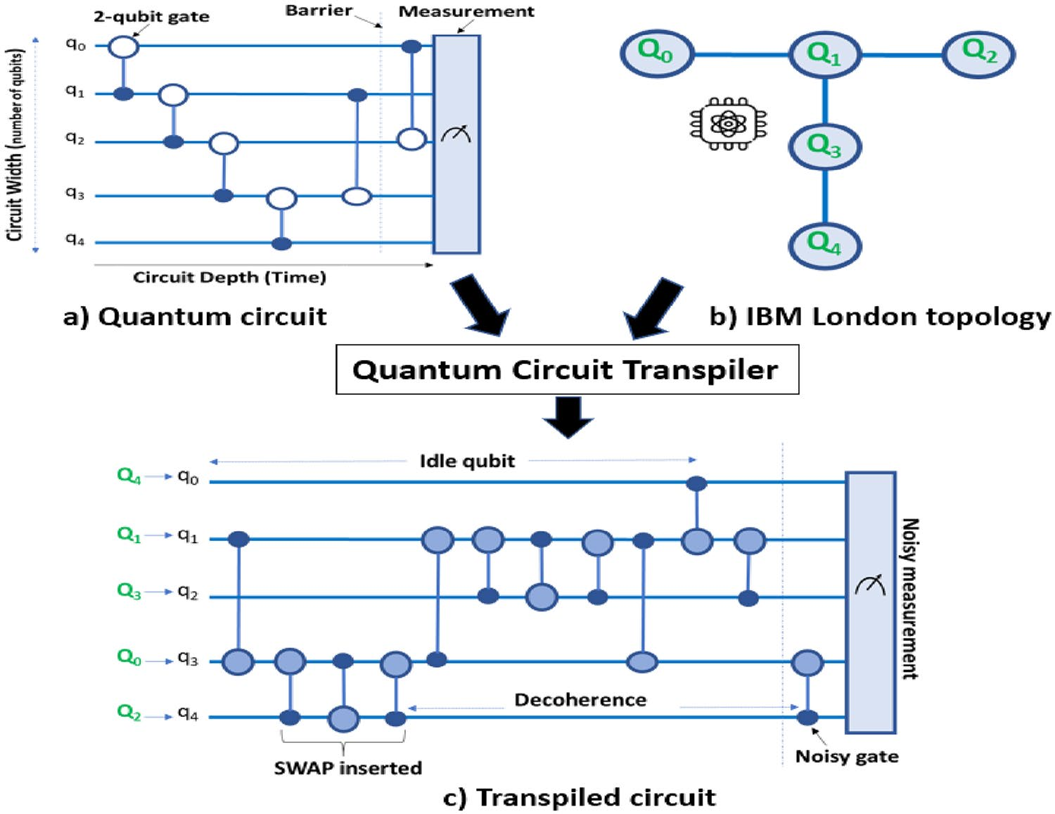
You write a quantum algorithm using abstract gates on abstract qubits. The hardware doesn’t speak that language. A real superconducting device (say, an IBM Eagle processor) has a fixed set of native gates — typically $\{R_z, \sqrt{X}, X, \text{CNOT}\}$ — and a constrained coupling map that dictates which pairs of physical qubits can directly interact. Transpilation is the process of bridging that gap. It happens in three stages:

Gate decomposition. Every gate in your algorithm is rewritten as a sequence of native gates. A Toffoli gate, for instance, breaks down into 6 CNOTs and several single-qubit rotations. This step is purely algebraic — no noise model involved.
Qubit mapping. Each logical qubit is assigned to a physical qubit on the device. A good mapping places qubits that interact frequently close together on the coupling graph.
Routing. When a two-qubit gate requires qubits that aren’t physically adjacent, the transpiler inserts SWAP gates to move qubit states along the coupling graph until the operands become neighbors.

A single SWAP gate costs 3 CNOTs. Every SWAP you insert is pure overhead — it performs no useful computation, only shuffles data so the next real gate can execute.

Here is the critical point: every stage adds gates, and every gate adds noise. Routing is the worst offender. On a device with limited connectivity (like a heavy-hex topology), even a modest circuit can require dozens of SWAPs.

A 10-qubit circuit on a heavy-hex device. Suppose your algorithm has 30 CNOT gates, but after routing, the transpiler inserts 50 SWAP gates. Each SWAP = 3 CNOTs, so that’s 150 extra CNOTs. With a typical two-qubit gate error rate of ~0.5%, the probability of no error across those 150 extra gates is $(1 - 0.005)^{150} \approx 47\%$. The routing overhead alone gives you a coin-flip chance of a completely clean execution — and that is before counting errors from the original gates.

Figure 1: The transpilation pipeline: a hardware-agnostic circuit is decomposed, mapped, and routed onto a physical device. Each step potentially increases the gate count and introduces noise.

Quantum Fidelity

Once we run a transpiled circuit on real hardware, we need a way to ask: how close is this noisy output to what the ideal circuit would have produced? This is what fidelity measures.

The basic setup: run your circuit many times (say, 8192 shots) and collect a probability distribution $Q_{\text{noisy}}$ over measurement outcomes. Compare it against the ideal distribution $P_{\text{ideal}}$ that you’d get from a perfect, noise-free simulation.

Hellinger fidelity. Given two discrete probability distributions $P$ and $Q$ over the same set of outcomes, the Hellinger fidelity is

\[F_H(P, Q) = \left(\sum_i \sqrt{P(i) \cdot Q(i)}\right)^2\]

$F_H = 1$ means the distributions are identical; $F_H = 0$ means they have no overlap at all.

Ideal 50/50 vs. noisy 55/45. Consider a single-qubit circuit that should produce $|0\rangle$ and $|1\rangle$ each with probability 0.5. Suppose the noisy device gives $P(0) = 0.55$ and $P(1) = 0.45$. Then:

\[F_H = \left(\sqrt{0.5 \times 0.55} + \sqrt{0.5 \times 0.45}\right)^2 = \left(\sqrt{0.275} + \sqrt{0.225}\right)^2\]

\[= (0.5244 + 0.4743)^2 = (0.9987)^2 \approx 0.9975\]

Not bad! But this is a trivially small circuit. As depth, gate count, and qubit count grow, fidelity drops — often rapidly. A fidelity below ~0.5 means the output is barely distinguishable from random noise.

Circuit Cutting

Here is the motivating question: what if your circuit needs more qubits than your device has? Or what if a large circuit accumulates so much transpilation noise that the output is useless? Circuit cutting offers an escape route: split the circuit into smaller pieces, run each piece independently, and reconstruct the full result classically.

There are two types of cuts:

Wire cuts sever a qubit wire between two gates. The qubit’s state at the cut point is decomposed into a set of basis states; the sub-circuits are each run with every possible boundary condition, and the results are stitched together.
Gate cuts remove an entangling gate (typically a CNOT) entirely. The gate’s action is decomposed into a set of local operations on each side of the cut, again requiring multiple executions with different configurations.

Wire cuts decompose a qubit state using the identity $\rho = \sum_i c_i \, \sigma_i$ over a quasi-probability basis. The coefficients $c_i$ can be negative — this is the “quasi” in quasi-probability.

The catch? Each cut multiplies the number of circuit executions you need. This is captured by the sampling overhead.

Sampling overhead. For $k$ cuts, the number of sub-circuit executions (and hence the classical post-processing cost) scales as:

Wire cuts: $\sim 4^k$
Gate cuts: $\sim 8^k$ (since a CNOT decomposes into more quasi-probability terms)

More precisely, to achieve the same statistical precision as running the full circuit once, you need $\mathcal{O}(4^k)$ or $\mathcal{O}(8^k)$ shots distributed across the various sub-circuit configurations.

BV circuit, 15 qubits, two different scenarios. A Bernstein-Vazirani circuit on 15 qubits has a simple, nearly linear entanglement structure — a chain of CNOTs. Suppose your device has a maximum width of 2 qubits (extreme, but illustrative):

You need 6 wire cuts to carve the circuit into 2-qubit pieces. Sampling overhead: $4^6 = 4{,}096$. Every shot of the original circuit now costs 4,096 sub-circuit executions.

Now suppose your device supports 5 qubits:

You only need 2 wire cuts to split into 5-qubit pieces. Sampling overhead: $4^2 = 16$.

That is a $256\times$ difference in classical cost, just from having a slightly larger device. The number of cuts dominates everything.

After running all sub-circuits, the results are combined via classical reconstruction: a linear algebra procedure that uses the quasi-probability coefficients to reassemble the full output distribution from the partial results.

Remark. The fundamental tension. This is the core tradeoff in circuit cutting: more cuts produce smaller sub-circuits that fit on smaller devices and accumulate less transpilation noise — but the classical reconstruction cost explodes exponentially with the number of cuts. Finding the sweet spot is the entire game, and it is exactly what DAScut is designed to do.

Interaction Density

Not all circuits are created equal. A Bernstein-Vazirani circuit has a tidy chain of CNOTs — cut the chain in a few places and you’re done. An efficiency circuit with all-to-all entanglement is a tangled web where every cut severs many connections. How do we quantify this difference?

DAScut introduces Interaction Density (ID), a single number that captures how entanglement-heavy a circuit is, weighted by the actual error rates of the device.

Interaction Density. For a sub-circuit partition $\pi$, the Interaction Density is

\[ID = \frac{W_2 \cdot n_{2g}^{(\pi)}}{W_2 \cdot n_{2g}^{(\pi)} + W_1 \cdot n_{1g}^{(\pi)}}\]

where $W_1$ is the average single-qubit gate error rate, $W_2$ is the average two-qubit gate error rate, $n_{1g}^{(\pi)}$ and $n_{2g}^{(\pi)}$ are the single- and two-qubit gate counts in the partition. ID ranges from 0 (no two-qubit gates) to 1 (all two-qubit gates, or single-qubit errors negligible).

The intuition: ID tells you what fraction of the total noise budget comes from entangling operations. A high ID means the circuit is dominated by two-qubit gate errors, which means cutting (which targets entangling gates) has a lot of noise to trade away — but also a lot of entanglement to sever, making cuts expensive.

ID values from the DAScut benchmarks. The authors report the following Interaction Densities for their test circuits:

Circuit	ID
BV (Bernstein-Vazirani)	0.88
Effi_circ (efficiency)	0.75
QAOA (optimization)	0.97

QAOA’s near-unity ID means almost all of its noise comes from two-qubit gates — it is densely entangled and hard to cut without massive overhead. BV, despite its high ID, has a linear entanglement structure that makes it easy to cut along natural boundaries. This is why DAScut considers both density and structure.

DAScut uses an ID threshold, $ID_{\max}$, as a decision boundary: if a circuit’s Interaction Density exceeds $ID_{\max}$, cutting is unlikely to help (the overhead will outweigh the noise reduction), and the circuit is better off running whole on the largest available device. Below the threshold, cutting is profitable and DAScut proceeds to find the optimal partition. We will see exactly how this threshold is calibrated in ?@sec-method.

Why Existing Approaches Fail

Circuit cutting sounds like a universal escape hatch: any circuit too large for your hardware can be sliced into smaller pieces, executed independently, and stitched back together classically. In practice, the escape hatch has a trap door. This section walks through three concrete ways that naive circuit cutting breaks down, using empirical data from Adufu & Kim (2026) to pin down when and why.

The Cutting Sensitivity Problem

Not every circuit responds to cutting the same way. Some circuits cut cleanly; others collapse. The difference comes down to entanglement structure, and you can see it starkly across four benchmark families.

Start with the Bernstein–Vazirani (BV) circuit. BV has a distinctive pattern: a single ancilla qubit interacts with each input qubit via CNOT, but the input qubits never interact with each other. Cut the circuit at width 2 (the smallest possible sub-circuit size), and fidelity is already 0.9648. Increase the sub-circuit width to 4 and fidelity hits a perfect 1.0, staying there at width 5, 6, and beyond. Fewer cuts means less classical overhead, and BV’s sparse entanglement structure means each cut severs very few quantum correlations.

BV at width 4. A 14-qubit BV circuit cut into sub-circuits of width 4 produces a fidelity of 1.0. That means the classically reconstructed output distribution is identical to the ideal quantum result. The circuit’s star-like interaction pattern means the cuts barely disturb the entanglement structure.

Now consider Effi_circ, a moderately entangled benchmark. At width 2, fidelity is exactly 0 — total failure. But as you increase the sub-circuit width, fidelity climbs: 0.1792 at width 4, 0.8789 at width 8, and 0.9993 at width 10. There is a sweet spot: cut too aggressively and you destroy the circuit’s correlations; cut too conservatively and you miss the point of cutting. Somewhere around width 8–10, the sub-circuits are large enough to preserve the circuit’s essential entanglement while still fitting on smaller hardware.

The story flips completely for Effi_full, which has dense all-to-all entanglement. Every qubit is entangled with every other qubit through a web of two-qubit gates. Cut this circuit anywhere, at any width, and the fidelity stays at 0. Width 2: zero. Width 4: zero. Width 10: zero. The reconstruction simply cannot recover the lost correlations. QAOA circuits behave similarly — their high-entanglement structure defeats every cutting strategy.

Remark. Remark. The key takeaway is that blindly cutting a circuit is dangerous. For BV, cutting is essentially free. For Effi_circ, it works only within a specific range of sub-circuit widths. For Effi_full and QAOA, no amount of cutting produces a usable answer. A framework that cannot distinguish these cases before committing to a cutting strategy will waste enormous resources on circuits it can never reconstruct.

Sampling Overhead Explosion

Even when cutting succeeds in principle, the classical cost can be staggering. Circuit cutting works by decomposing entangled operations across cut boundaries into a sum of separable channels. Each term in that sum requires independent sampling runs on the quantum hardware. The number of terms — the sampling overhead — grows exponentially with the number of cuts.

The concrete numbers from the paper make this visceral. Consider the BV circuit:

Sub-circuit width	Sampling overhead	Reconstruction time
2	531,441	379 s
3	6,561	7.5 s
4	144	1.2 s
5	9	0.2 s

More cuts (smaller sub-circuits) means exponentially more samples. But because BV has sparse entanglement, the overhead drops rapidly as you increase sub-circuit width. At width 5, only 9 samples are needed — trivial.

Now look at Effi_full:

Sub-circuit width	Sampling overhead	Reconstruction time
2	$3.28 \times 10^{93}$	—
4	$2.09 \times 10^{74}$	—
10	$5.15 \times 10^{47}$	$> 10^3$ s

A sampling overhead of $10^{93}$ means you would need more samples than there are atoms in the observable universe ($\approx 10^{80}$). This is not a practical difficulty — it is a physical impossibility.

Even at the most generous sub-circuit width (10 qubits), Effi_full requires $5.15 \times 10^{47}$ samples. The reconstruction is not merely expensive; it is computationally impossible. No classical machine will ever complete it. The fidelity numbers from the previous section (all zeros) are not just empirical observations — they reflect a fundamental barrier in the sampling overhead.

The correlation between sampling overhead and reconstruction time is direct and monotonic. For BV, reconstruction time drops from 379 seconds at width 2 to 0.2 seconds at width 5 — a 2000x improvement that mirrors the 60,000x reduction in sampling overhead. For Effi_full, reconstruction times stay in the thousands of seconds even at the largest sub-circuit widths, and the resulting output is still useless (fidelity 0).

Sampling overhead and the $4^k$ rule

The sampling overhead scales as $\bigO{4^k}$ where $k$ is the number of cuts. Each cut introduces a decomposition of one entangled channel into a sum of separable terms. For gate cuts (severing a two-qubit gate), each cut contributes a factor related to the Pauli basis decomposition. For wire cuts (severing a qubit wire), the factor involves teleportation-like channel decompositions. Either way, the exponential scaling in $k$ is unavoidable within the current circuit-cutting framework. DAScut does not eliminate this overhead — it avoids triggering it when the overhead would be catastrophic.

Device Heterogeneity

There is a third failure mode that has nothing to do with circuit structure: the choice of quantum device. The same circuit, with the same cutting strategy, produces different fidelities on different backends.

Same circuit, different devices. Take Effi_full at 14 qubits (no cutting — just direct execution). On IBM’s FakeMumbai backend, fidelity is 0.57. On FakeAuckland, fidelity jumps to 0.74. Both backends have 27 qubits. Both are based on IBM’s heavy-hex topology. The difference is in the noise profile: gate error rates, readout errors, $T_1$ and $T_2$ times, and crosstalk patterns all vary between devices.

This heterogeneity interacts with circuit cutting in a subtle way. When you cut a circuit, you generate sub-circuits that must be executed on some device. If you are distributing sub-circuits across multiple backends (as DAScut proposes), the choice of which sub-circuit runs on which device affects the overall fidelity. A sub-circuit that runs cleanly on one device might produce garbage on another, not because of anything wrong with the cutting strategy, but because the device’s native noise characteristics are unfavorable for that particular sub-circuit’s gate pattern.

Existing circuit cutting frameworks ignore this entirely. They cut the circuit, generate sub-circuits, and execute them on whatever backend is available — or on a single backend without considering whether a different device might produce better results. The scheduling decision (which sub-circuit goes where) is treated as a logistics problem, not a fidelity problem.

Remark. Remark. Device heterogeneity turns circuit cutting from a single optimization problem (how to cut) into a joint optimization problem (how to cut and where to run). Existing tools solve the first half and ignore the second. DAScut addresses both.

The Problem Statement

These three challenges — cutting sensitivity, sampling overhead explosion, and device heterogeneity — converge on a single question:

Problem statement. Given a quantum circuit too large for any available device, how can we (1) determine whether cutting is viable before committing resources, (2) minimize redundant execution of structurally identical sub-circuits, and (3) schedule sub-circuits across heterogeneous backends to maximize fidelity?

DAScut’s answer is a three-part framework: an interaction density metric that decides whether to cut, a canonicalization scheme that eliminates redundant sub-circuit executions, and a density- and structure-aware scheduler that matches sub-circuits to devices. The next section develops each component.

The DAScut Framework

DAScut tackles the three failure modes from the previous section with three matching components: an interaction density metric that decides whether to cut, a canonicalization scheme that eliminates redundant sub-circuit executions, and an algorithm that ties them together. This section develops each piece, starting from the concrete intuition and working toward the formal machinery.

Interaction Density: Deciding Whether to Cut

The first problem — cutting sensitivity — calls for a diagnostic. Before spending any resources on cutting, we need to know: will cutting this circuit produce a recoverable result? DAScut answers this with a single scalar: the interaction density (ID).

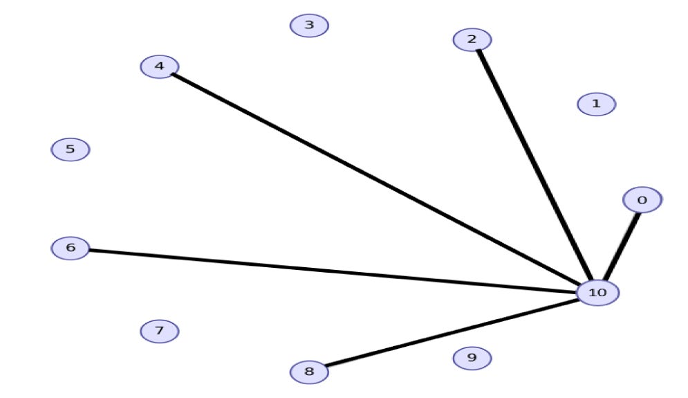
The idea is simple. Represent each qubit in the circuit as a node in a graph. Draw an edge between two nodes whenever those qubits interact via a two-qubit gate. The resulting structure is the circuit’s pair-wise interaction graph. Now look at the shape of that graph.

Interaction graphs showing dense vs. sparse pair-wise connectivity

A circuit like BV produces a star graph: one central node (the ancilla) connected to every other node, but no edges between the leaves. The graph is sparse — most qubit pairs never interact. Cutting this circuit means severing a few edges from the star’s center, which disrupts only a small fraction of the total entanglement.

A circuit like Effi_full produces something close to a complete graph: nearly every qubit interacts with every other qubit. The graph is dense — there is no clean place to cut. Any partition severs a large number of edges, and the classical reconstruction must account for all the lost correlations. This is what makes the sampling overhead explode.

Compare the interaction graphs visually: BV’s star has $n - 1$ edges for $n$ qubits. Effi_full’s near-complete graph has $\binom{n}{2} \approx n^2/2$ edges. The ratio grows linearly with circuit size.

The interaction density quantifies this distinction. It is the ratio of actual edges to possible edges in the interaction graph:

Interaction Density (ID). For a circuit on $n$ qubits with pair-wise interaction graph $G = (V, E)$:

\[ \text{ID} = \frac{|E|}{\binom{n}{2}} = \frac{2|E|}{n(n-1)} \]

The ID ranges from 0 (no two-qubit gates at all) to 1 (every qubit pair interacts).

Computing ID for BV and Effi_full. A 14-qubit BV circuit has 13 two-qubit interactions (each input qubit interacts with the ancilla). The maximum possible is $\binom{14}{2} = 91$. So $\text{ID}_{\text{BV}} = 13/91 \approx 0.14$. Sparse.

A 14-qubit Effi_full circuit has approximately 84 two-qubit interactions (nearly every pair). So $\text{ID}_{\text{Effi\_full}} = 84/91 \approx 0.92$. Dense.

DAScut uses a threshold $\text{ID}_\text{max}$: if a circuit’s interaction density exceeds this threshold, cutting is predicted to fail and the circuit should wait for a device large enough to run it monolithically. The experimental data from Section 3 supports this cleanly — circuits with low ID (BV, Effi_circ) respond well to cutting, while circuits with high ID (Effi_full, QAOA) do not.

Remark. Remark. The ID metric is deliberately coarse. It does not capture every nuance of entanglement structure (for instance, it does not distinguish between circuits with the same edge count but different topologies). What it does capture is the dominant effect: the density of two-qubit interactions is the primary predictor of cutting viability. A more refined metric could improve predictions at the margin, but ID already separates the “cuttable” from the “uncuttable” regimes with high accuracy.

Isomorphic Sub-Circuit Reuse

The second innovation is where DAScut gets clever. After cutting a circuit, you typically end up with many sub-circuits — potentially dozens or hundreds, depending on the number of partitions and the cutting strategy. The standard approach is to execute every single one of them on quantum hardware. DAScut observes that many of these sub-circuits are structurally identical, and you only need to run each unique structure once.

Why sub-circuits repeat

Think about what cutting does. It partitions a circuit along qubit boundaries, producing sub-circuits that each contain a subset of the original gates. Many quantum circuits have regular structure — repeated layers, symmetric gate patterns, uniform entangling blocks. When you cut such a circuit, the sub-circuits inherit that regularity. Two sub-circuits might operate on different physical qubits but apply exactly the same sequence of gates with the same parameters.

BV sub-circuits. Consider a BV circuit cut into sub-circuits of width 3. Each sub-circuit contains a Hadamard layer, a CNOT between the ancilla and one or two input qubits, and a measurement. Because every input qubit undergoes the same operations (just with different qubit labels), the resulting sub-circuits are structurally identical after relabeling. You might generate 5 sub-circuits, but only 1 is truly unique.

The challenge is making this observation precise. Two sub-circuits might look superficially different — different qubit register names, different gate decompositions from the transpiler, different qubit orderings — but be functionally identical. DAScut handles this through canonicalization: reducing every sub-circuit to a standard form so that structural equivalence becomes string equality.

The canonicalization pipeline

The canonicalization process has four steps:

Flatten to primitive gates. Decompose every gate into the basis set $\{rz, sx, x, cx, id\}$. This eliminates superficial differences from transpiler choices (e.g., one sub-circuit uses $R_y$ while another uses $sx \cdot rz \cdot sx$).
Remap to contiguous registers. Rename all qubit registers to a canonical form: $q[0], q[1], \ldots, q[n-1]$, assigned in order of first appearance. This eliminates differences in qubit labeling.
Normalize the QASM string. Produce the OpenQASM representation of the canonicalized circuit. Because the gate set and register names are now standardized, structurally identical circuits produce identical QASM strings.
Hash. Compute a hash of the normalized QASM string to produce a canonical key $K(c)$.

Isomorphic sub-circuits. Two sub-circuits $c_1$ and $c_2$ are isomorphic if they produce the same canonical key: $K(c_1) = K(c_2)$. Isomorphic sub-circuits apply the same sequence of primitive gates in the same topology, differing only in qubit labels and possibly gate-library presentation.

Reuse efficiency. Given a set of sub-circuits with $N_\text{total}$ elements, of which $N_\text{exec}$ are unique representatives:

\[ \text{Reuse}_\text{eff} = \frac{N_\text{total} - N_\text{exec}}{N_\text{total}} \times 100\% \]

A reuse efficiency of 90% means only 10% of sub-circuits need to be executed on quantum hardware.

Effi_circ reuse. The paper reports that Effi_circ achieves up to 97.36% reuse efficiency. Out of all generated sub-circuits, only about 2.6% are structurally unique. The rest are duplicates that can be identified via canonicalization and skipped entirely. This translates directly into a $$38x reduction in quantum hardware usage.

Canonicalization details

The canonicalization procedure is deterministic: the same sub-circuit always produces the same canonical key, regardless of the qubit naming scheme or gate library used by the transpiler. The key property that makes this sound is register-order invariance: by assigning canonical register names in order of first gate appearance, two sub-circuits that apply the same gates to “corresponding” qubits (even if those qubits have different original names) will map to the same key.

Consider two sub-circuits:

Sub-circuit A: cx q_3, q_7; rz(0.5) q_7; sx q_3
Sub-circuit B: cx q_0, q_1; rz(0.5) q_1; sx q_0

After remapping (step 2), both become: cx q[0], q[1]; rz(0.5) q[1]; sx q[0]. After flattening (step 1, already in basis), normalizing (step 3), and hashing (step 4), both produce the same key $K$.

The DAScut Algorithm

With interaction density and isomorphic reuse in hand, we can now walk through the full DAScut algorithm. The procedure takes a quantum circuit and a set of available backends as input, and produces an execution plan that either runs the circuit directly or cuts it intelligently.

Algorithm 1: DAScut

Input: Quantum circuit $C$, set of available backends $\mathcal{B}$

Output: Execution results (reconstructed probability distribution)

Direct execution check. If $C$ fits on any backend $b \in \mathcal{B}$ (i.e., the circuit’s qubit count $\leq$ the device’s qubit count), execute $C$ directly on the best available device. Return the result. No cutting needed.
Get recommended cuts. Call Qiskit’s partition_problem() on $C$ to obtain a set of recommended cut locations. These are the qubit wires or gates where the circuit can be partitioned with minimal entanglement disruption.
Cut and partition. Apply the cuts to $C$, producing a set of sub-circuits $\{s_1, s_2, \ldots, s_m\}$ organized by partition label $\ell$. Each partition label groups sub-circuits that belong to the same fragment of the original circuit.
Canonicalize and deduplicate. For each sub-circuit $s_i$:
1. Compute the canonical key $K(s_i)$ using the four-step pipeline (flatten, remap, normalize, hash).
2. If $K(s_i)$ matches an existing representative, mark $s_i$ as a duplicate and store a pointer to the representative.
3. If $K(s_i)$ is new, register $s_i$ as a new representative.
Calculate reuse savings. Compute $\text{Reuse}_\text{eff}$ and report the number of unique sub-circuits that actually require execution.
Execute representatives. Run only the unique representative sub-circuits on quantum hardware. For duplicates, copy the results from their representative.
Reconstruct. Combine all sub-circuit results (executed and copied) using the classical reconstruction procedure to recover the full circuit’s output distribution.

Walkthrough with a 14-qubit BV circuit. Suppose we have two backends, each with 7 qubits. The 14-qubit BV circuit does not fit on either, so step 1 fails. Step 2 identifies cut locations along the ancilla’s connections. Step 3 produces, say, 8 sub-circuits across 2 partitions. Step 4 canonicalizes all 8 and discovers that 6 of them are duplicates of 2 unique representatives. Step 5 reports $\text{Reuse}_\text{eff} = 75\%$. Step 6 executes only the 2 unique sub-circuits. Step 7 reconstructs the full 14-qubit output using the 2 executed results (each reused 3 times).

The algorithm’s time complexity is linear in the total number of sub-circuits: $\bigO{\sum_\ell m_\ell}$, where $m_\ell$ is the number of sub-circuits in partition $\ell$. The canonicalization step (step 4) dominates, but it involves only string operations (flattening, renaming, hashing) that run in time proportional to sub-circuit size. No exponential blowup, no combinatorial search.

Remark. Remark. Step 1 is more important than it looks. The interaction density check (from Section 4.1) can be folded into this step: if the circuit does not fit on any device and its ID exceeds $\text{ID}_\text{max}$, DAScut can report early that cutting is unlikely to succeed. This prevents the framework from wasting resources on circuits like Effi_full where cutting is futile regardless of strategy.

Why Canonicalization Works for Circuit Cutting

There is a subtlety worth pausing on. In general quantum computing, two circuits that apply the same gates to corresponding qubits are not guaranteed to produce the same output — because the output depends on the input state, which may differ. If circuit A operates on qubits that start in $\ket{01}$ and circuit B operates on qubits that start in $\ket{10}$, isomorphic structure tells you nothing about output equivalence.

Circuit cutting is different. When a circuit is cut, the sub-circuits at each cut boundary receive a fixed, protocol-determined set of input states: the Pauli eigenstates $\{\ket{0}, \ket{1}, \ket{+}, \ket{-}, \ket{+i}, \ket{-i}\}$. These boundary states are dictated by the cutting decomposition, not by the original circuit’s input. Every sub-circuit, regardless of where it sits in the original circuit, receives the same set of boundary conditions.

This means that isomorphic sub-circuits do not just look the same — they produce identical measurement results. The canonical key is not merely a structural fingerprint; it is a functional fingerprint. Two sub-circuits with the same $K(c)$ will return the same probability distributions for every boundary-state configuration in the cutting protocol.

Remark. Remark. This property is specific to circuit cutting and does not hold for quantum computing in general. If you were running sub-circuits as standalone programs with user-specified inputs, isomorphic structure would not guarantee identical outputs. It is the fixed boundary conditions of the cutting protocol that make deduplication sound. This is what makes circuit cutting uniquely suited for canonicalization-based optimization — a happy accident of the protocol’s mathematical structure.

Fidelity-Aware Scheduling

So far, DAScut has done two things: it looked at a circuit’s entanglement structure and decided whether cutting is worth it (Interaction Density), and it identified duplicate sub-circuits after cutting so it can run each one only once (isomorphic reuse). But there is a third question that existing frameworks punt on entirely: which device should each sub-circuit actually run on?

This matters more than you might think. Today’s quantum cloud platforms are not a single monolithic machine. They are fleets of heterogeneous QPUs — each with its own qubit count, gate error rates, readout fidelities, and coherence times. A 7-qubit sub-circuit that runs cleanly on a low-noise 14-qubit backend might produce garbage on a noisier 27-qubit machine, even though both devices have enough qubits. Assigning sub-circuits to the first available device — which is what most schedulers do — leaves fidelity on the table.

The scheduling problem

Here is the setup. You have a queue of circuits submitted by one or more users. Each circuit has been through DAScut’s density analysis and cutting stages, producing a collection of sub-circuits. You also have a set of heterogeneous QPUs, each characterized by its noise profile (gate errors, readout errors, coherence times) and its capacity (number of qubits, maximum circuit depth before decoherence kills you). The goal: assign every sub-circuit to a device and schedule execution to minimize total makespan — the wall-clock time from the first sub-circuit starting to the last one finishing — while keeping fidelity as high as possible.

These two objectives conflict. The fastest schedule might route everything to the largest device (maximizing parallelism), but that device might be the noisiest. The highest-fidelity schedule might route everything to the quietest device, but that device might be small, forcing serial execution and ballooning the makespan. DAScut resolves this trade-off with a single tunable metric.

Fidelity-aware device mapping

Utility cost. For a given sub-circuit $s$ and candidate device $d$, the utility cost is

\[U(s, d) = \alpha \, T_{\text{norm}} + (1 - \alpha)(1 - F_{\text{est}})\]

where $T_{\text{norm}}$ is the normalized expected runtime of $s$ on $d$ (computed via ALAP scheduling), $F_{\text{est}}$ is the estimated execution fidelity of $s$ on $d$, and $\alpha \in [0, 1]$ balances speed against fidelity. Lower $U$ means a better device for this sub-circuit.

The fidelity estimate $F_{\text{est}}$ is not a single number pulled from a vendor dashboard. It is a product of every noise source the sub-circuit will encounter:

\[F_{\text{est}} = (1 - e_1)^{n_1} \times (1 - e_2)^{n_2} \times (1 - e_{\text{ro}})^{n_{\text{ro}}} \times e^{-T/T_2} \times e_c^{K}\]

where $e_1$ and $e_2$ are the single- and two-qubit gate error rates, $n_1$ and $n_2$ are the corresponding gate counts, $e_{\text{ro}}$ is the readout error rate applied $n_{\text{ro}}$ times, $T/T_2$ captures decoherence over the circuit’s execution time relative to the device’s $T_2$ coherence time, and $e_c^K$ accounts for $K$ additional error channels (crosstalk, leakage, etc.).

Picking a device. Suppose you have a sub-circuit with Interaction Density $ID = 0.75$ — moderately dense, with a fair number of two-qubit gates. You set $\alpha = 0.3$ because fidelity matters more than speed for this workload.

Device A (14 qubits, low noise): $T_{\text{norm}} = 0.8$, $F_{\text{est}} = 0.92$. $U_A = 0.3 \times 0.8 + 0.7 \times (1 - 0.92) = 0.24 + 0.056 = 0.296$
Device B (27 qubits, higher noise): $T_{\text{norm}} = 0.4$, $F_{\text{est}} = 0.78$. $U_B = 0.3 \times 0.4 + 0.7 \times (1 - 0.78) = 0.12 + 0.154 = 0.274$
Device C (14 qubits, very low noise): $T_{\text{norm}} = 0.9$, $F_{\text{est}} = 0.96$. $U_C = 0.3 \times 0.9 + 0.7 \times (1 - 0.96) = 0.27 + 0.028 = 0.298$

Device B wins on raw utility, but only because it is fast enough to compensate for its noise. If you increase $\alpha$ toward 0.1 (heavily favoring fidelity), Device C with its 0.96 fidelity pulls ahead. The point: $\alpha$ gives the scheduler — or the user — a knob to express priorities.

The $\alpha$ parameter is not just a mathematical convenience. In practice, a VQE user running hundreds of parameter-sweep iterations might set $\alpha = 0.7$ (prioritize throughput), while a user running a single high-precision simulation might set $\alpha = 0.2$ (prioritize fidelity).

Iso-aware deduplication in scheduling

There is a subtlety in when isomorphic deduplication happens relative to scheduling, and getting the order right matters.

After cutting but before scheduling, DAScut scans all sub-circuits across all jobs in the queue — not just within a single circuit. It identifies isomorphic sub-circuits using the canonical-form comparison from the previous section, groups them into equivalence classes, and marks all but one representative per class as “reuse.” Only the representatives enter the scheduling pipeline.

This is particularly powerful for homogeneous workloads: parameter sweeps, VQE iterations, or batches of structurally identical circuits with different rotation angles. In these settings, many circuits share the same skeleton, and cutting them produces sub-circuits that are identical up to qubit relabeling. In DAScut’s experiments, a batch of 10 EfficientSU2 circuits produces 4,752 sub-circuits before deduplication — and just 462 after. That is 90.27% fewer circuits entering the scheduler, which directly translates to less time spent solving the scheduling optimization and less time occupying QPU resources.

MILP-based scheduling

Once deduplication has shrunk the set of sub-circuits to unique representatives, DAScut formulates the scheduling problem as a Mixed Integer Linear Program (MILP). The MILP minimizes total makespan subject to two types of constraints: device capacity (a QPU can only run circuits that fit within its qubit count, and only so many at once) and precedence (some sub-circuits depend on the results of others for classical reconstruction, so they must execute in the right order).

Why MILP?

MILP is a natural fit for scheduling problems where decisions are discrete (which device? what time slot?) but the objective is continuous (minimize makespan). The solver explores the space of valid assignments and finds the optimal — or near-optimal — schedule. The key insight for DAScut: because iso-aware deduplication has already reduced the number of sub-circuits by up to 90%, the MILP instance is much smaller than it would be for a naive scheduler. Fewer variables and constraints mean faster solving, which is critical when the scheduler itself is on the critical path.

The full workflow

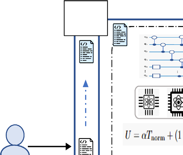
Putting it all together, here is what happens when a batch of circuits hits DAScut.

Figure 2: DAScut execution workflow. Circuits enter the pipeline, undergo density analysis and fidelity-aware device mapping, are cut (if appropriate), deduplicated via isomorphism detection, scheduled via MILP onto heterogeneous QPUs, executed, and reconstructed.

Submit. Circuits enter the queue, each tagged with its qubit count and gate list.
Density analysis. DAScut computes $ID$ for each circuit. Dense circuits ($ID > \tau$) are deferred to a device large enough to run them uncut.
Fidelity-aware mapping. Each sub-circuit is scored against every available QPU using the utility cost $U$. The best device is recorded.
Circuit cutting. Circuits that passed the density filter are cut to fit the target device width, using Qiskit’s wire-cutting decomposition.
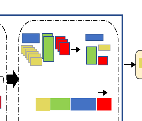
Iso-aware deduplication. All sub-circuits across all jobs are flattened, compared, and grouped. Only unique representatives survive.
MILP scheduling. Representatives are assigned to devices and time slots to minimize makespan.
Execute. Representatives run on their assigned QPUs.
Reconstruct. Results are mapped back to all isomorphic copies, and the full probability distributions are classically reconstructed.

Remark. Notice that steps 3–6 form a pipeline where each stage reduces the work for the next. Density filtering removes circuits that should not be cut. Cutting produces sub-circuits. Deduplication shrinks the sub-circuit set. MILP optimizes the schedule over the reduced set. Each stage makes the next one cheaper — a design that compounds efficiency gains rather than adding them linearly.

Results

Engineering a pipeline is one thing. Does it actually deliver? This section unpacks DAScut’s experimental evaluation in two settings: single-circuit execution (where the focus is on fidelity and reuse efficiency) and multi-circuit scheduling (where makespan, throughput, and scalability take center stage).

All experiments use IBM’s FakeMelbourne backend — a 14-qubit simulated device with a realistic noise model derived from actual hardware calibration data. The benchmark circuits span four families: Bernstein-Vazirani (BV), EfficientSU2 with circular entanglement (Effi_circ), EfficientSU2 with full entanglement (Effi_full), and QAOA. These were chosen to cover the spectrum from sparse (BV) to dense (QAOA), exercising DAScut’s density-aware logic across its full range.

Single-circuit execution

The first question: when DAScut cuts a single circuit and reconstructs the result, how much fidelity do you lose, and how many sub-circuits can isomorphic reuse eliminate?

Reuse efficiency

Reuse efficiency measures the fraction of sub-circuits that are structurally redundant — isomorphic to another sub-circuit and therefore skippable. Higher is better; 100% would mean every sub-circuit is a duplicate (which never happens in practice because you need at least one unique representative).

The results vary dramatically by circuit type:

Effi_circ achieves reuse efficiencies of up to 97.36% at width 2. This circuit has a circular entanglement pattern — each qubit talks to its neighbor in a ring — which produces highly regular sub-circuits after cutting. Nearly all of them are isomorphic.
BV achieves reuse of 51–79%, depending on the cut width. BV is sparse and structured (a fan of CNOT gates from one ancilla to all data qubits), so many sub-circuits share the same topology, but the asymmetry between the ancilla side and the data side limits perfect reuse.
Effi_full and QAOA achieve reuse of near 0%. These circuits are densely entangled — every qubit interacts with many others — so cutting them produces sub-circuits with diverse internal structures. There are few duplicates to exploit.

This is exactly why Interaction Density matters as a pre-filter. Dense circuits like Effi_full and QAOA are poor candidates for cutting and poor candidates for reuse. DAScut’s density check catches them before the pipeline wastes effort.

Fidelity analysis

Figure 3 tells the fidelity story, and it has two distinct chapters.

Sparse circuits hold up well. BV and Effi_circ maintain fidelities in the range of 0.85–0.98 across circuit widths from 6 to 15 qubits. The cutting overhead is present but manageable: reconstructed fidelity is consistently lower than running the circuit uncut on a device large enough to hold it, because each cut introduces a classical sampling overhead that adds noise. But the gap is small enough to be practical.

Dense circuits collapse. Effi_full and QAOA show reconstructed fidelities near zero for circuits wider than about 8 qubits. This is not a bug in DAScut — it is the fundamental physics of circuit cutting. A densely entangled circuit requires many cuts, each of which demands exponentially more samples to reconstruct the correlations that were severed. For Effi_full at width 10, cutting requires 98 cuts, producing a sampling overhead of $\sim 3.28 \times 10^{93}$. No amount of clever scheduling can rescue that.

Remark. The fidelity results validate DAScut’s decision to not cut dense circuits. The Interaction Density filter exists precisely because dense circuits produce garbage after reconstruction. Deferring them to a larger device — even if that means waiting in a longer queue — is always the right call.

Noisy vs. noiseless reconstruction. When DAScut reconstructs the probability distribution, it uses measurement results from noisy hardware. The reconstructed fidelity is therefore strictly lower than the ideal (noiseless) reconstruction. Across all benchmarks, the noisy reconstructed fidelity tracks about 2–5% below the noiseless version for sparse circuits. For dense circuits, both are near zero, so the distinction is academic.

Why QAOA is the hardest case

QAOA (Quantum Approximate Optimization Algorithm) circuits are designed to explore the full Hilbert space of a combinatorial problem. Their entanglement pattern is deliberately dense: the “cost layer” applies $ZZ$-interactions between all pairs of qubits connected in the problem graph, and the “mixer layer” applies single-qubit rotations to all qubits. This all-to-all interaction structure means that cutting anywhere severs correlations that carry problem-specific information. The result: high Interaction Density, near-zero reuse efficiency, and fidelity collapse after reconstruction. QAOA is the poster child for circuits that should run uncut on a large enough device.

Multi-circuit scheduling

The real payoff of DAScut’s pipeline comes when you have many circuits to schedule across multiple devices. Here, density filtering, isomorphic deduplication, and fidelity-aware mapping work in concert to slash makespan and boost throughput.

DAScut is compared against two baselines:

SeqSched: sequential scheduling. Each circuit is cut and executed one at a time, in order. No cross-circuit optimization.
MILQ: a state-of-the-art bin-packing scheduler that packs sub-circuits onto devices to minimize idle time, but without density awareness or isomorphic reuse.

Homogeneous workload

The homogeneous benchmark consists of 10 Effi_circ circuits with qubit counts ranging from 10 to 15. This is the kind of workload you see in parameter sweeps or VQE iterations: structurally similar circuits submitted as a batch.

Sub-circuit reduction. This is where iso-aware deduplication shines.

Figure 4: Sub-circuit comparison across schedulers for the homogeneous workload. DAScut’s iso-aware deduplication reduces the sub-circuit count by 90.27%.

DAScut: 462 sub-circuits
MILQ: 4,752 sub-circuits
SeqSched: 4,752 sub-circuits

That is a 90.27% reduction in the number of sub-circuits that actually need to execute. MILQ and SeqSched both execute every sub-circuit independently — they have no mechanism to detect that most of them are structurally identical.

Makespan.

DAScut: 315.92 s
MILQ: 10,710 s
SeqSched: 2,746 s

DAScut finishes the entire batch in about 5 minutes. SeqSched takes 46 minutes. MILQ takes nearly 3 hours — slower than the sequential baseline — because its bin-packing overhead is not recouped by any sub-circuit reduction.

Figure 5: Normalized speedup for the homogeneous workload. DAScut achieves 8.69x speedup over the SeqSched baseline. MILQ actually slows down to 0.26x.

Normalized speedup (relative to SeqSched):

DAScut: 8.69x
MILQ: 0.26x (slower than baseline)

Reading the speedup numbers. A speedup of 8.69x means DAScut completes the workload in $1/8.69 \approx 11.5\%$ of the time that SeqSched takes. MILQ’s 0.26x means it takes $1/0.26 \approx 3.85$ times longer than the baseline. The scheduling overhead of MILQ’s bin-packing, applied to 4,752 sub-circuits, overwhelms any parallelism gains. DAScut’s MILP scheduler works on only 462 sub-circuits, so its optimization overhead is small relative to the execution time saved.

Throughput.

DAScut: 30 circuits per 1,000 s
SeqSched: 3 circuits per 1,000 s
MILQ: 1 circuit per 1,000 s

DAScut processes circuits at 10x the rate of the sequential baseline and 30x the rate of MILQ.

Heterogeneous workload

The heterogeneous benchmark is harder: 10 different circuits drawn from VQE, BV, GHZ, Linear Chain (LC), QAOA, Effi_circ, and Effi_full. These circuits have different structures, densities, and sizes — a realistic model of a shared quantum cloud queue.

Sub-circuit count.

DAScut: 1,185 sub-circuits
MILQ: 2,456 sub-circuits

A 51.7% reduction — less dramatic than the homogeneous case, because heterogeneous circuits share fewer isomorphic sub-circuits.

Makespan.

DAScut: 1,256 s
MILQ: 7,998 s

An approximately 6x speedup. DAScut completes the heterogeneous batch in 21 minutes; MILQ takes over 2 hours.

Reuse efficiency across circuit types. The heterogeneous workload reveals how reuse efficiency depends on circuit structure:

Effi_circ: 92.3% (circular entanglement = highly regular sub-circuits)
BV: 65–79% (sparse, structured)
GHZ, LC: 40–55% (moderate regularity)
VQE: 20–35% (parameterized rotations reduce symmetry)
Effi_full, QAOA: ~0% (dense, irregular)

Average across the batch: 52%.

Fidelity-aware placement. DAScut’s utility-cost-based device mapping improves fidelity by 3–5 $\times$ 10$^{-3}$ compared to noise-unaware placement. This is a modest but consistent gain: it comes for free as part of the scheduling pipeline, and it compounds over many circuits in a batch.

Key correlations

The paper reports a correlation analysis (Table 7) that quantifies the relationships between circuit properties and system-level performance. Three numbers stand out:

Table 1: Key correlations between circuit properties and performance metrics.

Correlation	Value
Reuse efficiency $\leftrightarrow$ throughput	+0.89
Interaction Density $\leftrightarrow$ fidelity	+0.73
Interaction Density $\leftrightarrow$ throughput	-0.82

High reuse drives high throughput (+0.89): the fewer unique sub-circuits you need to execute, the faster the batch finishes. Higher density correlates with higher fidelity (+0.73) — but only because dense circuits are deferred to larger devices and run uncut, preserving their fidelity. And higher density kills throughput (-0.82): dense circuits cannot be cut efficiently, cannot benefit from reuse, and occupy device resources for longer.

Remark. The sweet spot for DAScut. High reuse efficiency and low Interaction Density. Circuits with regular, sparse entanglement patterns — parameter sweeps of variational circuits, repeated motifs in error correction, families of structured algorithms — are where DAScut delivers its largest gains. Dense, irregular circuits are better served by running uncut on large devices, and DAScut is smart enough to route them there.

Summary of key results

Table 2: Summary of DAScut’s performance across homogeneous and heterogeneous workloads.

Metric	DAScut	MILQ	SeqSched
Sub-circuits (homogeneous)	462	4,752	4,752
Makespan, homogeneous (s)	315.92	10,710	2,746
Speedup vs SeqSched	8.69x	0.26x	1.0x
Throughput (circuits / 1000 s)	30	1	3
Makespan, heterogeneous (s)	1,256	7,998	—
Sub-circuits (heterogeneous)	1,185	2,456	—
Avg. reuse efficiency (hetero.)	52%	0%	0%

Outlook

What DAScut proves

The central claim of DAScut is not that circuit cutting works — that was established years ago. The claim is that structure-awareness is essential for making circuit cutting practical.

Consider what happens without it. A structure-blind scheduler takes a 15-qubit circuit, cuts it into sub-circuits that fit on a 14-qubit device, and executes all of them. If the circuit is sparse (like BV), this works fine but wastes resources: many sub-circuits are duplicates that could have been skipped. If the circuit is dense (like QAOA), the blind approach produces thousands of sub-circuits with astronomical sampling overhead — and the reconstructed result is garbage anyway. Either way, the scheduler does not know which situation it is in until after it has committed resources.

DAScut proves that two simple structural analyses — Interaction Density as a pre-filter and isomorphic detection as a post-filter — can transform circuit cutting from an indiscriminate tool into a selective one. The density check prevents you from cutting circuits that will not survive reconstruction. The isomorphism check prevents you from executing sub-circuits whose results you already have. Together, they reduce sub-circuit counts by 90% on favorable workloads and eliminate futile cuts on unfavorable ones.

“Structure-aware” is not a vague aspiration. In DAScut, it means two concrete, computable quantities: Interaction Density and graph isomorphism. Both are polynomial-time checks that run before any quantum hardware is touched.

Limitations

DAScut is an early-stage system, and the authors are candid about its boundaries.

Simulated backends only. All experiments run on IBM’s Fake* devices — noise models derived from real hardware calibration data, but not real hardware. Simulated noise is stationary and well-characterized; real noise drifts, exhibits crosstalk, and surprises you with correlated errors that no simple product model captures. The fidelity estimates that drive DAScut’s device mapping ($F_{\text{est}}$) assume independent error channels; on real hardware, this assumption will be approximate at best.

GPU memory caps simulation scale. The classical reconstruction of cut circuits requires computing and combining exponentially many sub-circuit results. The experiments are limited to 14-qubit circuits (the FakeMelbourne backend) because the classical post-processing exceeds GPU memory for larger widths. This is not a limitation of DAScut’s algorithm — the density analysis, cutting, and scheduling stages scale to arbitrary circuit sizes — but it limits the experimental validation to modest qubit counts.

Fixed density threshold. The Interaction Density threshold $\tau$ that separates “cut-worthy” from “defer to a larger device” is set as a fixed constant. In principle, the optimal threshold depends on the workload mix, the available devices, and the user’s fidelity-vs-speed preference. An adaptive threshold — one that adjusts based on queue pressure, device availability, or historical performance — could improve utilization but is left to future work.

Inherent fidelity penalty. Circuit cutting is not free. Every cut introduces a classical sampling overhead, and the reconstructed distribution is always noisier than what you would get by running the uncut circuit on a large-enough device. DAScut mitigates this by avoiding unnecessary cuts (density filtering) and reducing the number of noisy executions (reuse), but it cannot eliminate the fundamental overhead of the quasi-probability decomposition.

Broader context

DAScut occupies an interesting position in the quantum computing stack.

At one end of the spectrum, tools like Chipmunq (Bandic et al., 2025) target the fault-tolerant regime: they compile QEC-encoded circuits onto chiplet architectures, preserving the patch geometry that error correction requires. Chipmunq’s problem is “this logical circuit is too big for one chiplet” — and its solution is structure-preserving placement and routing across chiplet boundaries.

At the other end, near-term NISQ users submit raw circuits to cloud platforms and hope for the best. Their problem is “this circuit is too wide for any single device I can access” — and their solution, if they have one, is ad-hoc circuit cutting without structural guidance.

DAScut sits between these two worlds. It targets NISQ-era circuits (no error correction, no logical qubits), but it brings the same structural insight that makes Chipmunq effective: do not ignore the internal structure of what you are compiling. Chipmunq preserves QEC patches; DAScut preserves entanglement-sparse regions. Both deal with “too big for one chip,” but at different abstraction levels and for different hardware eras.

DAScut vs. Chipmunq: same insight, different layers

Both papers appeared in the same research area and share a core architectural insight: structure-blind compilation destroys the thing you are trying to compute. For Chipmunq, that thing is the QEC code structure — breaking a surface code patch inflates logical error rates by 128x. For DAScut, it is the sparsity pattern of the circuit — cutting a dense circuit produces an exponential blowup in sampling overhead. The lesson generalizes: any compilation tool that treats its input as an opaque bag of gates will waste resources or produce garbage (or both) once the input has exploitable structure.

Future directions

Real hardware validation. The most important next step is running DAScut on actual QPUs — IBM’s Eagle and Heron processors, IonQ’s trapped-ion systems, or Quantinuum’s H-series devices. Real hardware will stress-test the fidelity model, the density threshold, and the iso-detection pipeline in ways that simulation cannot.

Time-varying calibration data. Current noise models are static snapshots. Real device error rates drift over minutes to hours. A production version of DAScut should ingest live calibration data and update both the Interaction Density calculation and the utility cost function in real time, re-routing sub-circuits away from devices whose noise has spiked since the last calibration cycle.

Adaptive density threshold. Instead of a fixed $\tau$, the threshold could be learned from historical execution data: which circuits at which density levels produced acceptable fidelity after reconstruction? A Bayesian or reinforcement-learning approach could tune $\tau$ per circuit family, per device, or per workload mix.

Integration with error mitigation. DAScut currently does not apply error mitigation (zero-noise extrapolation, probabilistic error cancellation, etc.) to its sub-circuit results. Combining cutting with mitigation could recover some of the fidelity lost to the cutting overhead, potentially extending DAScut’s useful range to moderately dense circuits that are currently deferred.

How DAScut compares

Table 3: Feature comparison of circuit-cutting schedulers. DAScut is the only system that combines structural analysis, isomorphic reuse, and fidelity-aware device mapping.

	DAScut	MILQ	SeqSched
Structure-aware	Yes (ID metric)	No	No
Iso-reuse	Yes	No	No
Fidelity-aware scheduling	Yes	No	No
Speedup vs. baseline	8.69x	0.26x	1.0x

MILQ is a capable bin-packing scheduler, but it operates on the output of circuit cutting without questioning whether cutting was the right choice or whether the resulting sub-circuits are redundant. SeqSched is the naive baseline — cut and execute, one at a time. DAScut’s advantage comes not from a single trick but from the compounding effect of three structure-aware stages: density filtering reduces the circuits that enter cutting, iso-detection reduces the sub-circuits that enter scheduling, and fidelity-aware mapping ensures those sub-circuits run on the best available hardware.

Remark. An honest assessment. DAScut’s gains are largest on structured, sparse workloads — exactly the circuits where cutting is viable in the first place. For dense, irregular circuits, DAScut’s contribution is knowing not to cut them, which is valuable but less dramatic. The open question is whether the structured-circuit sweet spot covers enough of the workloads that real quantum cloud users submit. If the future of quantum computing is dominated by variational algorithms with regular ansatz structures (VQE, QAOA on sparse graphs, quantum machine learning), DAScut’s approach has legs. If it is dominated by arbitrary, dense circuits, the density filter will route everything to large devices, and DAScut reduces to a fidelity-aware scheduler without the cutting and reuse stages. Either way, the structural analysis costs almost nothing to compute — so there is no penalty for checking.