NALAC: Efficient Routing for Logical Entangling Gates on Zoned Neutral Atom Architectures
A self-contained walkthrough of arXiv:2405.08068
Introduction
Neutral atom quantum computers can rearrange their qubits mid-computation. Lasers grab individual atoms, shuttle them across the chip, and drop them next to whichever partner they need to interact with — all in microseconds. This extraordinary flexibility should make routing trivial compared to fixed-connectivity platforms like superconducting chips. In practice, it does not. The moment you scale to fault-tolerant circuits, where each logical qubit is a block of dozens or hundreds of physical qubits, the routing problem comes roaring back — and none of the existing tools were built to handle it.
This paper (arXiv: 2405.08068) was published in 2024 by researchers at the Technical University of Munich, working within the Munich Quantum Toolkit (MQT).
Two problems collide
To see why, we need two pieces of context.
Problem 1: Logical qubits are not points — they are arrays. Fault-tolerant quantum computing encodes each logical qubit into a block of physical qubits using a quantum error-correcting code. A Steane code uses 7 physical qubits; a distance-\(d\) surface code uses \(\mathcal{O}(d^2)\). A transversal logical CZ gate between two Steane-encoded qubits requires performing a physical CZ gate between every corresponding pair of physical qubits — all 7 pairs simultaneously. The atoms are not individual points to be moved around; they are rigid arrays that must be shuttled as units while preserving their internal geometry.
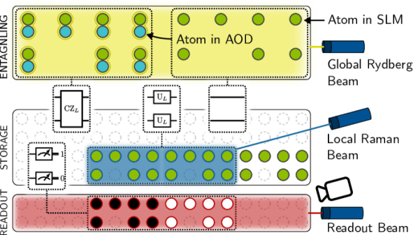
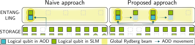
Problem 2: Zoned architectures impose subtle movement constraints. State-of-the-art neutral atom hardware, following the pioneering work of Bluvstein et al. (2024), separates the chip into functional zones: an entangling zone where global Rydberg pulses execute CZ gates, a storage zone where qubits wait in low-noise SLM traps, and a readout zone for mid-circuit measurements. Atoms move between zones on acousto-optic deflector (AOD) rails — but AOD rows and columns cannot cross, ghost trapping spots at grid intersections must be avoided, and the two interacting arrays cannot both sit in the AOD at once. These constraints interact in non-obvious ways, and violating any one of them produces garbage.
Bluvstein et al. and the dawn of zoned architectures
In late 2023, a Harvard-led team demonstrated a zoned neutral atom processor executing fault-tolerant circuits on up to 48 logical qubits. Their key innovation was physically separating entangling, storage, and readout into different spatial regions, connected by atom shuttling. This experiment was a watershed moment for neutral atom quantum computing, and it defined the architectural template that NALAC targets. The NALAC paper provides the first formal computational model for this class of hardware.
What NALAC does
NALAC (Neutral Atom Logical Array Compiler) attacks this problem in three steps:
- Model — It formalizes the zoned architecture into an abstract computational model, identifying four precise shuttling constraints that any valid routing solution must satisfy.
- Route — Given a set of logical entangling gates, it constructs an interaction graph and uses a modified graph-coloring algorithm (based on DSatur) to schedule gates into parallel batches while respecting all movement constraints.
- Position — It computes exact physical coordinates for every qubit at every time step, translating the abstract schedule into concrete shuttling instructions.
The result is a polynomial-time compiler that maximizes gate parallelism and minimizes the time atoms spend in transit.
Results at a glance
Across a benchmark suite of 16 circuit families from the MQT Bench library (all at 20 logical qubits), NALAC achieves:
- Up to 84% reduction in routing overhead compared to the naive serialized approach — for instance, QFT drops from 139 \(\mu\)s to 22 \(\mu\)s, and QNN from 266 \(\mu\)s to 57 \(\mu\)s.
- Up to 3.7 parallel CZ gates per Rydberg pulse, exploiting the fact that a global beam can entangle multiple well-separated pairs simultaneously.
- Millisecond-scale compilation times even for circuits with 20+ logical qubits, keeping the tool practical for iterative design workflows.
Remark. Remark. The parallelism gains are uneven across circuit families. Circuits like QNN and QPE, which have dense, regular entanglement patterns, benefit enormously (3.6–3.7x parallelism). Circuits like QFT and Deutsch-Jozsa, whose entanglement structure is more sequential, see modest parallelism gains (1.0x) but still benefit from reduced shuttling distances. The routing overhead reduction, however, is consistently large across all families.
Roadmap
We begin with the background needed to follow the paper: neutral atom hardware, transversal gates, and the shuttling mechanism (Section 2). Next, we formalize the zoned architecture model and its four constraints (Section 3). We then walk through the NALAC routing algorithm step by step (Section 4), followed by the position computation that turns an abstract schedule into physical coordinates (Section 5). Finally, we examine the evaluation results (Section 6) and discuss limitations and future directions (Section 7).
Background
Before diving into NALAC’s architecture model and routing algorithm, we need three pieces of background: how neutral atom hardware works, why fault tolerance turns individual atoms into rigid arrays, and how the entangling zone actually executes gates. If you are already comfortable with these topics, skip ahead to Section 3.
Neutral atom quantum computing
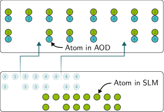
In a neutral atom quantum computer, individual atoms — typically rubidium-87 or ytterbium-171 — are trapped by tightly focused laser beams called optical tweezers. Each atom encodes one physical qubit in two of its internal energy levels. The defining feature of this platform is reconfigurability: atoms can be physically moved during a computation by adjusting the laser beams that hold them.
Optical tweezers. There are two types of traps. SLM traps (spatial light modulator) are static: the laser pattern is fixed, creating a nearly arbitrary but immovable array of trapping sites. AOD traps (acousto-optic deflector) are dynamic: the deflector steers a laser beam along two axes, creating a movable 2D lattice of traps. By adjusting AOD frequencies, entire rows and columns of atoms can be repositioned in parallel.
The interplay between SLM and AOD traps is central to everything that follows. SLM traps provide stable, long-term storage — atoms parked in them experience minimal noise and can hold their quantum state for milliseconds or longer. AOD traps provide the mobility needed to bring atoms together for entangling operations. A typical cycle looks like this: pick up atoms from SLM traps using the AOD, shuttle them to the entangling zone, perform gates, and return them to SLM storage.
Think of SLM traps as parking spots and AOD traps as a forklift that moves atoms between spots.
Entangling gates via Rydberg interaction
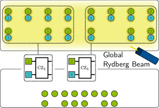
Two-qubit entangling gates on neutral atom platforms exploit the Rydberg blockade. When an atom is excited to a high-energy Rydberg state, it creates a strong dipole field that shifts the energy levels of nearby atoms, preventing them from being simultaneously excited. This conditional behavior implements a controlled-Z (CZ) gate: the two-atom system picks up a phase of \(\pi\) if and only if both atoms are in the \(\ket{1}\) state.
Global Rydberg pulse. In a zoned architecture, the entangling zone is illuminated by a global Rydberg beam. When activated, it attempts to excite every atom in the zone. Atoms that are close enough to each other (within the blockade radius) undergo a CZ interaction. Atoms that are isolated — far from any neighbor — simply perform an identity operation. The gate duration is approximately 0.2 \(\mu\)s.
This is a crucial point: the Rydberg beam is not targeted at specific pairs. It hits everything in the entangling zone. The compiler’s job is to position the atoms so that exactly the desired pairs are close enough to interact, while all other atoms are safely far apart. If two atoms that should not interact end up within the blockade radius, the computation is corrupted.
Parallel gates in action. Suppose we have four logical qubits \(q_1, q_2, q_3, q_4\) and we want to execute CZ(\(q_1, q_2\)) and CZ(\(q_3, q_4\)) simultaneously. We position \(q_1\) next to \(q_2\) and \(q_3\) next to \(q_4\), but with sufficient spacing between the two pairs. A single Rydberg pulse then executes both CZ gates in parallel. The overhead is the time to position the atoms, not the gate itself.
Fault tolerance and transversal gates
A single physical qubit is far too noisy for useful computation. Quantum error correction encodes one logical qubit across multiple physical qubits, using a code that can detect and correct errors. The Steane code encodes one logical qubit into 7 physical qubits; color codes and surface codes use larger arrays.
The key property that makes neutral atoms attractive for fault tolerance is transversal gate execution. A transversal gate applies the same physical operation to each corresponding pair of physical qubits in two encoded blocks, independently and in parallel.
Transversal CZ gate. Given two logical qubits \(q_A^L\) and \(q_B^L\), each encoded in \(n\) physical qubits, the transversal CZ gate executes \(\text{CZ}(q_A^{(i)}, q_B^{(i)})\) for \(i = 1, \ldots, n\) simultaneously. Because each physical gate acts on a separate pair, errors cannot spread from one physical qubit to another within the same block — the gate is inherently fault-tolerant.
For a Steane code (\(n = 7\)), a transversal logical CZ requires 7 physical CZ gates in parallel. For a distance-3 color code, it might be 9 or more. The atoms are arranged in a logical array — a fixed spatial pattern matching the code’s geometry — and the two arrays must be brought into precise overlap so that every corresponding pair falls within the Rydberg blockade radius.
Transversal gates alone are not universal — you also need non-transversal operations like magic state injection. But transversal CZ gates are the workhorse for most fault-tolerant circuits.
This is where the routing problem originates. We cannot just move individual atoms; we must shuttle entire arrays as rigid units, align them precisely, and then separate them — all while obeying the hardware’s movement constraints.
The routing challenge
Given a fault-tolerant circuit with \(k\) logical qubits and a sequence of logical CZ gates, the routing problem is: determine, for each gate, when to execute it and where to place the two interacting arrays in the entangling zone, such that:
- All gates execute correctly (the right pairs interact, no unintended interactions).
- All shuttling constraints are satisfied (no AOD crossings, no ghost spots).
- The total execution time — dominated by atom movement, not gate duration — is minimized.
The naive approach serializes everything: execute one logical CZ gate at a time, moving exactly two arrays into the entangling zone per cycle. This is correct but slow. NALAC’s contribution is to parallelize gate execution within each cycle while respecting all hardware constraints, reducing the overall routing overhead by 30–57%.
The Zoned Architecture Model
The central contribution of this paper is not just a routing algorithm — it is the formalization of the architecture itself. Before NALAC, there was no abstract model of zoned neutral atom hardware that captured the constraints precisely enough to build a compiler on top of. Let’s walk through this model piece by piece.
Zones and their roles
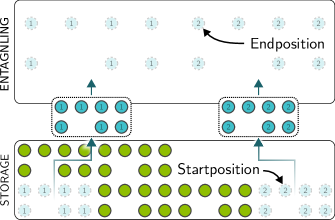
The architecture partitions the physical space into three functionally distinct regions:
Zoned architecture. A zoned neutral atom architecture consists of:
- Entangling zone — illuminated by a global Rydberg beam. All atom pairs within the blockade radius undergo a CZ interaction. Isolated atoms perform the identity.
- Storage zone — atoms rest in static SLM traps with high coherence. Single-qubit gates can be executed here. No entangling operations occur.
- Readout zone — dedicated to qubit measurement. Fluorescence imaging can determine the state of atoms here without disturbing qubits in other zones.
The physical separation is not merely organizational — it is necessary. The Rydberg beam that enables entangling gates would corrupt stored qubits if they were in the same region. Similarly, the fluorescence imaging used for measurement would decohere nearby qubits. By placing these operations in isolated spatial zones, the architecture protects qubits not currently involved in a gate.
The readout zone enables mid-circuit measurement, which is essential for error correction syndrome extraction and feed-forward operations.
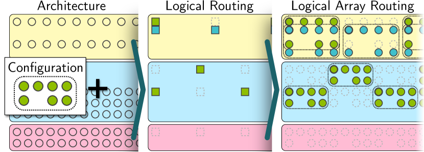
Logical qubit arrays
Each logical qubit is encoded as a fixed spatial arrangement of physical atoms — a logical array. The shape and size of the array depend on the error-correcting code:
| Code | Physical qubits | Array shape |
|---|---|---|
| Steane code | 7 | \(2 \times 4\) (with one vacancy) |
| Distance-3 color code | 9 | \(3 \times 3\) |
| Distance-5 surface code | 25 | \(5 \times 5\) |
The internal geometry of the array is rigid — the atoms within a logical qubit maintain fixed relative positions throughout the computation. What changes is the position of the array as a whole as it is shuttled between zones.
The four shuttling constraints
Here is where the model earns its keep. The AOD mechanism that moves atoms imposes four constraints, and getting any one of them wrong means the routing solution is physically unrealizable.
Let’s take them one at a time.
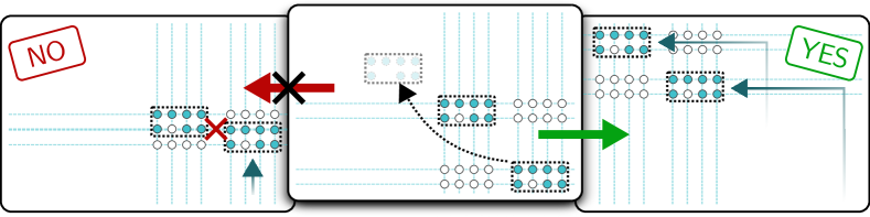
(a) Row-column non-crossing. AOD rows and columns must maintain a minimum separation and cannot swap their relative order during movements. If row \(A\) is above row \(B\) at the start of a movement, row \(A\) must remain above row \(B\) at the end. The same applies to columns.
This constraint arises because AOD frequencies determine row/column positions, and the frequencies must remain ordered to avoid ambiguity in the trapping potential.
(b) Row-column preservation. If two atoms share the same AOD row (or column) at any point, they continue sharing it throughout the movement. The AOD moves entire rows and columns as units, not individual atoms. You can think of it as a grid printed on a sheet of rubber — you can stretch or compress the rows and columns, but you cannot detach an atom from its row.
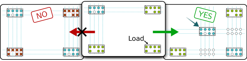
(c) Ghost-spot avoidance. The AOD creates traps at every intersection of its row and column beams, not just the positions where we intend to place atoms. These unintended trapping sites — called ghost spots — can capture stray atoms or disturb atoms that happen to be in SLM traps at those coordinates. The routing solution must ensure that ghost spots do not overlap with any occupied SLM trap positions.
Why ghost spots are dangerous. Suppose the AOD has two active rows at positions \(y_1\) and \(y_2\), and two active columns at \(x_1\) and \(x_2\). This creates four trapping sites: \((x_1, y_1)\), \((x_1, y_2)\), \((x_2, y_1)\), \((x_2, y_2)\). We may only want atoms at two of these positions, but the other two are also trapping-capable. If an SLM-held atom happens to sit at one of these ghost spots, it can be disturbed or pulled out of its static trap.
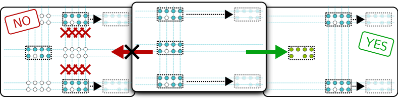
(d) Array alignment. To execute a transversal logical CZ gate, the two interacting arrays must physically overlap so that corresponding qubit pairs are within the Rydberg blockade radius. Critically, only one of the two arrays can be in the AOD during this overlap — the other must be placed in SLM traps. If both arrays were in the AOD, moving them into overlap would violate the non-crossing constraint (their rows and columns would have to merge).
Remark. Remark. Constraint (d) is the most consequential for the routing algorithm. It means that for every CZ gate, NALAC must decide which of the two arrays is the “mover” (held in the AOD) and which is the “stayer” (placed in SLM traps in the entangling zone). This binary choice per gate is what links the routing problem to graph coloring, as we will see in Section 4.
A single execution cycle
Putting it all together, one execution cycle — which the paper calls a run — proceeds as follows:
- Load: Transfer selected qubit arrays from SLM storage traps to AOD traps. Duration: ~20 \(\mu\)s per load operation.
- Shuttle: Move the AOD-held arrays from the storage zone to the entangling zone.
- Position: Arrange atoms so that intended interaction partners are within blockade radius and all others are far apart.
- Execute: Fire the global Rydberg pulse. All valid pairs undergo CZ. Duration: ~0.2 \(\mu\)s.
- Reposition (optional): If multiple gate batches are scheduled within the same run, rearrange atoms for the next batch and fire again.
- Return: Shuttle arrays back to storage and transfer from AOD to SLM traps. Duration: ~20 \(\mu\)s per store.
The dominant cost is movement, not gate execution. A CZ gate takes 0.2 \(\mu\)s, but loading and shuttling take 20 \(\mu\)s each. This is why minimizing the number of runs and the shuttling distance within each run is the central optimization target.
Routing overhead. The routing overhead is the total additional time spent on atom movement (loading, shuttling, and storing) beyond what would be needed if all gates could be executed instantaneously in place. It excludes gate execution time. NALAC’s goal is to minimize this quantity.
The Routing Algorithm
With the architecture model in hand, we can now tackle the core algorithmic question: given a set of logical CZ gates to execute, how do we schedule them into parallel batches and assign the mover/stayer roles, all while respecting the four shuttling constraints?
NALAC’s approach is elegant: reduce the routing problem to a constrained graph-coloring problem on an interaction graph, and solve it with a modified version of the DSatur algorithm.
The interaction graph
The first step is to identify which gates are currently executable — meaning all their predecessor operations in the circuit have already been completed (or commute with the current gate, so order does not matter).
Interaction graph. Given a quantum circuit, the interaction graph \(G = (V, E)\) at any point in the execution is defined as:
- \(V\) = the set of logical qubits involved in at least one currently executable entangling gate
- \(E\) = the set of currently executable entangling gates, where edge \((q_i, q_j) \in E\) iff a CZ gate between \(q_i\) and \(q_j\) is executable
The interaction graph is undirected (CZ is symmetric) and changes as gates are executed.
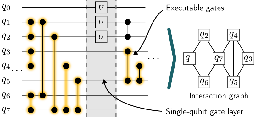
The interaction graph is rebuilt after each run, as executing gates makes new ones become executable.
Independent sets and the mover/stayer partition
Recall constraint (d): for each CZ gate, one array must be in the AOD (the mover) and the other in SLM traps (the stayer). If a qubit is the mover for multiple gates in the same run, it stays in the AOD the entire time and is sequentially positioned next to different stayer partners.
This leads to a natural partition. We want to find a set of qubits that will be the movers — held in the AOD — such that no two movers interact with each other (which would require both to be in SLM, contradicting their mover role). In graph theory terms, we need an independent set.
Independent set. A subset \(I \subseteq V\) of the interaction graph is an independent set if no two nodes in \(I\) are adjacent. Nodes in \(I\) become AOD-held movers; nodes in \(V \setminus I\) become SLM-held stayers.
A small example. Consider an interaction graph with four qubits and edges: \((q_1, q_2)\), \((q_1, q_3)\), \((q_2, q_4)\). The set \(\{q_1, q_4\}\) is an independent set: neither \(q_1\) nor \(q_4\) shares an edge. Choosing them as movers means \(q_1\) (in the AOD) will sequentially visit \(q_2\) and \(q_3\) (both in SLM traps), while \(q_4\) (also in the AOD) visits \(q_2\). All three gates can be executed in one run.
NALAC computes a maximal independent set using a greedy heuristic: sort nodes by degree (descending) and iteratively add nodes that are not adjacent to any already-selected node. The choice of high-degree nodes first is deliberate — a mover with many neighbors can cover many gates in a single run.
Finding the maximum independent set is NP-hard, but the greedy maximal independent set is computed in \(\mathcal{O}(|V| + |E|)\) time and is empirically sufficient.
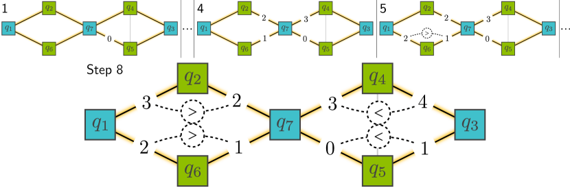
Constrained edge coloring with modified DSatur
Once we know which qubits are movers (AOD) and which are stayers (SLM), we need to determine the order in which gates execute within a single run. Each mover must visit its stayer partners in some sequence, and we need to ensure that the non-crossing constraint is never violated during these movements.
NALAC formulates this as an edge coloring problem. Each edge in the interaction graph (incident to a mover node) receives a color — an integer representing its execution time step. Two edges sharing a node must receive different colors (a standard edge-coloring requirement). But there is an additional constraint specific to the AOD:
AOD ordering constraint (Constraint C). For any two mover nodes \(u, v \in I\) and any path of length 2 between them (i.e., \(u - w - v\) where \(w\) is a stayer), the color ordering must be consistent: the colors on the two edges must both increase toward the same endpoint. Formally, if \(c(u,w) < c(v,w)\), then for any other stayer \(w'\) on a length-2 path between \(u\) and \(v\), we must also have \(c(u,w') < c(v,w')\).
Why does this constraint exist? Because movers travel left-to-right (or right-to-left) through the line of stayers. If mover \(u\) visits stayer \(w\) before mover \(v\) does, then \(u\) must be to the left of \(v\) relative to \(w\). For this left-right ordering to be consistent across all shared stayers, the color ordering must be monotone. Violating this would require two AOD rows to cross — exactly what constraint (a) forbids.
The paper solves this with a modified DSatur algorithm:
Algorithm: Modified DSatur Edge Coloring
Input:  Interaction graph G = (V, E), Independent set I ⊆ V
Output: Coloring c: E → ℕ

1. Initialize all edges as uncolored
2. For each mover v ∈ I (sorted by degree, descending):
3.    For each edge e incident to v (sorted by saturation,
      then degree):
4.       Assign e the least color that is:
         (i)  different from all colors on adjacent edges
         (ii) consistent with Constraint C: larger than any
              color on an adjacent edge of a different mover
              sharing the same stayer
5. Return coloring cRemark. Remark. The standard DSatur algorithm colors nodes; NALAC adapts it to color edges, with the additional monotonicity constraint. The greedy strategy (process high-degree movers first, assign the smallest valid color) tends to produce compact colorings with few distinct time steps, which directly translates to fewer repositioning operations within a run.
From coloring to schedule
The coloring directly yields the execution schedule:
- Color 0: All edges colored 0 execute first. Each mover is positioned next to its color-0 stayer partner. The Rydberg pulse fires.
- Color 1: Movers reposition to their color-1 partners. Rydberg pulse fires again.
- Continue until all colors are exhausted.
After all gates in the current interaction graph are executed, NALAC rebuilds the interaction graph (new gates may have become executable) and repeats the process. The algorithm terminates when no executable gates remain.
Walking through a run. Suppose the coloring assigns three colors (0, 1, 2) to a run with 3 movers and 7 gates. At step 0, all 3 movers execute one gate each (3 parallel CZ gates). At step 1, 2 movers have a second partner; 2 more parallel CZ gates. At step 2, 1 mover has a third partner; 1 final CZ gate. Total: 7 gates executed in 3 Rydberg pulses, with only 2 repositioning movements between pulses. The naive approach would have needed 7 separate runs.
Position Computation
The coloring algorithm tells us when each gate executes and who moves. But it does not tell us where to place each atom. That is the job of the position computation stage — and it must produce exact physical coordinates that satisfy all four shuttling constraints simultaneously.
Ordering the stayer qubits
The stayer qubits (those in SLM traps in the entangling zone) must be arranged in a line. The order of this line is not arbitrary — it is dictated by the coloring.
For each mover \(v\), the coloring assigns an ordering to \(v\)’s stayer neighbors: the stayer with color 0 is visited first, then color 1, then color 2, and so on. Because the mover travels left-to-right (to avoid backtracking, which would risk AOD crossings), the stayers must be placed in this order along the line.
When multiple movers are active, each imposes its own ordering on the stayers it visits. These orderings may overlap — two movers might both visit the same stayer — but the AOD ordering constraint (Constraint C from Section 4.3) guarantees that the orderings are compatible. They can be combined into a single consistent total ordering.
Stayer partial order. For each mover \(v \in I\), define a directed path through \(v\)’s stayer neighbors in the order of their edge colors: \(w_0 \to w_1 \to w_2 \to \cdots\). The union of all such directed paths defines a partial order on the stayer qubits. A topological sort of this partial order yields a valid left-to-right placement.
The compatibility of these orderings is precisely what Constraint C guarantees. Without it, the partial order could contain cycles, making a valid placement impossible.
Placing the movers
Mover qubits (held in the AOD) are assigned positions between the stayer qubits. At each time step, a mover must be adjacent to its current interaction partner — close enough for the Rydberg blockade to take effect. At all other times, it must be far enough from every stayer to avoid unintended interactions.
The algorithm assigns each mover a sequence of positions:
- Active position: directly next to the stayer it is interacting with at this time step.
- Resting position: a safe location between two stayers, outside the blockade radius of both, used during time steps when the mover has no scheduled gate.
Resting positions. Suppose stayers are placed at \(x\)-coordinates 0, 10, 20, 30 (in units of the inter-array spacing). A mover interacting with the stayer at position 10 during step 1 would be placed at \(x = 10\) (overlapping for the CZ gate). During step 2, if it has no gate, it moves to a resting position at \(x = 15\) — safely between the stayers at 10 and 20, too far from either to trigger a Rydberg interaction.
Putting it together: a complete run
Let’s walk through the full position computation for one run, using the interaction graph from the earlier examples.
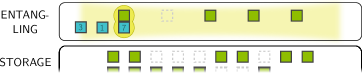
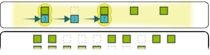
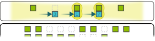
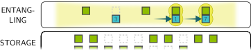
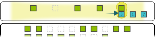
Five time steps of a complete execution run. SLM-held stayer qubits remain fixed in the entangling zone. AOD-held mover qubits shuttle left-to-right between partners. At each step, pairs within the blockade radius undergo CZ gates via the global Rydberg pulse.
At \(t = 0\):
- All stayers are placed in SLM traps in the entangling zone, ordered by the topological sort.
- All movers are loaded into the AOD from storage.
At \(t = 1\):
- Each mover moves to its color-0 partner. The Rydberg pulse fires. CZ gates execute for all mover-stayer pairs that are adjacent.
- Movers without a color-0 gate park at resting positions.
At \(t = 2\):
- Movers shift right to their color-1 partners. Another Rydberg pulse. More CZ gates.
- The left-to-right progression ensures no AOD rows cross.
This continues until all colors are exhausted, at which point the movers are returned to storage and the next run begins.
Scaling to physical coordinates
So far we have described positions at the logical level — each node in the interaction graph represents a logical qubit array. The final step is to scale these logical positions to physical coordinates.
Each logical array occupies a rectangular region whose size depends on the error-correcting code (e.g., \(2 \times 4\) for Steane, \(5 \times 5\) for distance-5 surface code). The inter-array spacing must be large enough that atoms in adjacent arrays do not accidentally interact via the Rydberg mechanism.
Physical position mapping. Given a logical position \(x_L\) for a qubit array and an array size of \(a_x \times a_y\) atoms with inter-atom spacing \(\delta\), the physical position of the \((i,j)\)-th atom in the array is: \[ (x_{phys}, y_{phys}) = (x_L \cdot s_x + i \cdot \delta, \; y_L \cdot s_y + j \cdot \delta) \] where \(s_x, s_y\) are the logical-to-physical scaling factors ensuring sufficient inter-array separation.
Remark. Remark. Larger error-correcting codes require larger arrays, which in turn require more physical space in the entangling zone and longer shuttling distances. This is a fundamental trade-off: stronger error correction demands more physical resources and longer routing overhead. The evaluation in Section 6 quantifies this trade-off explicitly.
Evaluation
The authors evaluate NALAC against a naive baseline on benchmark circuits from the MQT Bench library, measuring three things: routing overhead, gate parallelism, and compilation time. Let’s walk through each.
Experimental setup
Benchmarks. 16 circuit families from MQT Bench, including QAOA, VQE, QFT, QNN, QPE, GHZ, graph states, Deutsch-Jozsa, and several parameterized ansatz circuits. All circuits are first transpiled to the neutral atom native gate set: local and global rotations plus CZ gates.
Hardware model. Based on the Bluvstein et al. experimental setup:
| Parameter | Value |
|---|---|
| Load/store duration | 20 \(\mu\)s |
| Shuttling speed | 0.55 \(\mu\)m/\(\mu\)s |
| CZ gate duration | 0.2 \(\mu\)s |
| Logical qubits | 20 (default) |
The 20 \(\mu\)s load/store time dominates the routing overhead. A single CZ gate takes only 0.2 \(\mu\)s — two orders of magnitude less.
Baseline. The naive approach serializes all gates: one logical CZ gate per run, with exactly two arrays moving into the entangling zone each time. No parallelism, no batching.
Machine. Apple M3 with 16 GB RAM.
RQ1: Routing overhead reduction
How much time does NALAC save on atom shuttling?
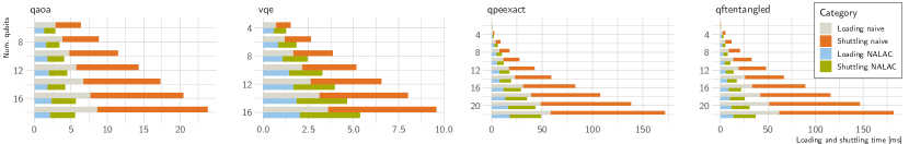
The headline results are dramatic. Here is a selection from the full table (all at 20 logical qubits):
| Circuit | CZ gates | Naive overhead (\(\mu\)s) | NALAC overhead (\(\mu\)s) | Avg. parallel CZ |
|---|---|---|---|---|
| QNN | 778 | 266 | 57 | 3.6 |
| QPE (exact) | 406 | 139 | 43 | 3.7 |
| QFT | 408 | 139 | 22 | 1.0 |
| QFT entangled | 429 | 147 | 31 | 2.8 |
| Graph state | 20 | 7 | 1 | 3.3 |
| AE | 380 | 130 | 32 | 1.1 |
| Portfolio VQE | 570 | 195 | 31 | 1.0 |
The savings come from two sources:
- Fewer runs. By batching multiple gates into a single run, NALAC eliminates redundant load/store cycles. Each load/store pair costs 40 \(\mu\)s; eliminating even a few runs saves hundreds of microseconds.
- Shorter shuttling distances. By arranging stayers intelligently and having movers travel in one direction, NALAC avoids the back-and-forth shuttling that the naive approach requires.
Concrete numbers. For a QNN circuit with 20 logical qubits:
- Naive routing overhead: 266 \(\mu\)s
- NALAC routing overhead: 57 \(\mu\)s
- Reduction: 79%
For QFT:
- Naive: 139 \(\mu\)s
- NALAC: 22 \(\mu\)s
- Reduction: 84%
RQ2: Gate parallelism
How many CZ gates does NALAC execute per Rydberg pulse?
The global Rydberg beam can entangle multiple pairs simultaneously, but only if they are correctly positioned. NALAC’s coloring algorithm directly optimizes for this.
| Circuit family | Avg. parallel CZ gates per pulse |
|---|---|
| QNN | 3.6 |
| QPE (exact) | 3.7 |
| Graph state | 3.3 |
| AE | 1.1 |
| QFT | 1.0 |
| DJ | 1.0 |
Remark. Remark. The variation is entirely explained by the circuit’s entanglement structure. QNN and QPE circuits have many commuting CZ gates that can be batched together. QFT circuits have a sequential fan-out structure where each qubit interacts with all subsequent qubits — there is less room for parallelism. But even at 1.0 gates per pulse, NALAC still wins on shuttling distance.
RQ3: Compilation time
Does NALAC scale?
A compiler that produces optimal schedules but takes hours to run is useless for iterative design. NALAC’s polynomial-time algorithms keep compilation fast:
- All 20-qubit benchmarks compile in under 100 milliseconds.
- Scaling to larger circuits shows polynomial growth, remaining in the millisecond range even as qubit count increases.
- The greedy independent set and DSatur coloring are both near-linear in graph size.
Compare this to qubit-level compilers like LightSABRE, which can time out on circuits with thousands of physical qubits. NALAC’s logical-level abstraction keeps the problem tractable.
RQ4: Impact of array size
What happens as we increase the error-correcting code distance?
Larger codes mean larger logical arrays, which mean more physical space per qubit and longer shuttling distances. The paper evaluates array sizes from \(1 \times 1\) (bare physical qubits, for reference) up to \(7 \times 7\) (distance-7 surface code scale).
Key findings:
- Loading time stays roughly constant. Arrays are loaded in parallel regardless of size, and the load operation time is dominated by the fixed 20 \(\mu\)s trap transfer.
- Shuttling time increases linearly with array size. Larger arrays need more physical space, so atoms travel farther between positions. The shuttling speed (0.55 \(\mu\)m/\(\mu\)s) is fixed.
- Fewer logical qubits fit per row. As arrays grow, the entangling zone accommodates fewer qubits side by side, which can force additional runs.
Scaling from Steane to surface codes. With 7-qubit Steane arrays (\(2 \times 4\)), a 20-qubit circuit’s routing overhead might be 266 \(\mu\)s. With \(5 \times 5\) distance-5 surface code arrays, the same circuit’s overhead grows to roughly 500–600 \(\mu\)s, driven almost entirely by the longer shuttling distances. The NALAC-vs-naive ratio remains similar, but the absolute overhead climbs with code size.
RQ5: Architecture design impact
How does the storage zone layout affect performance?
The paper compares two architecture variants:
- Wide storage zone: storage is broad, allowing many qubits to be placed close to the entangling zone boundary.
- Narrow storage zone: storage is elongated, forcing some qubits to travel farther to reach the entangling zone.
The narrow layout increases both loading and shuttling times, because:
- Qubits farther from the zone boundary take longer to shuttle.
- Fewer qubits fit in each row of the storage zone, requiring more loading steps.
Remark. Remark. This result highlights that NALAC is not just a compiler — it can also serve as an architecture evaluation tool. By parameterizing the zone layout and array sizes, designers can use NALAC to explore the performance implications of different hardware configurations before committing to a fabrication run.
Discussion and Outlook
NALAC is the first tool to formalize and solve the routing problem for logical qubit arrays on zoned neutral atom architectures. But it is a first step, not the last word. Let’s discuss what it achieves, what it assumes, and where the field goes next.
Naive vs. NALAC: a quantitative snapshot
| Metric | Naive | NALAC | Improvement |
|---|---|---|---|
| Routing overhead (QNN, 20 qubits) | 266 \(\mu\)s | 57 \(\mu\)s | 79% reduction |
| Routing overhead (QFT, 20 qubits) | 139 \(\mu\)s | 22 \(\mu\)s | 84% reduction |
| Max parallel CZ per pulse | 1.0 | 3.7 | 3.7\(\times\) |
| Compilation time | ms | ms | Similar |
The gains are substantial and consistent. But notice what is not in this table: logical error rates. NALAC minimizes routing time but does not explicitly optimize for noise — it does not steer operations away from noisier regions or balance decoherence budgets.
Limitations
1. Transversal gates only. NALAC handles transversal CZ gates, which are the workhorse of fault-tolerant circuits but are not sufficient for universality. A universal gate set also requires non-transversal operations — typically magic state injection and distillation — which involve complex multi-round protocols that do not fit the current model.
Magic state distillation is one of the most resource-intensive components of fault-tolerant quantum computing, often consuming the majority of physical qubits.
2. Greedy heuristics, not optimal solutions. The maximal independent set and DSatur coloring are greedy algorithms with polynomial runtime. They produce good solutions quickly, but there is no guarantee of optimality. For small instances, an exact solver might find tighter schedules — but the millisecond compilation times make the greedy approach practical for the iterative design workflows that hardware teams need.
3. Static architecture model. The model assumes a fixed zone layout with known dimensions. It does not account for dynamic reconfiguration of the zones themselves, time-varying noise profiles, or real-time feedback from measurement outcomes.
4. No noise-aware optimization. Unlike chiplet-aware compilers (e.g., Chipmunq, which explicitly penalizes noisy inter-chiplet links), NALAC treats all CZ gates as equally costly. In reality, atoms that travel farther may experience more decoherence, and incorporating distance-dependent noise into the cost function could improve logical error rates.
Open challenges
Non-transversal gate integration. Extending the model to handle magic state injection, lattice surgery, and other non-transversal operations would make NALAC applicable to full fault-tolerant circuits. This likely requires a richer zone model with dedicated distillation regions.
Noise-aware routing. Incorporating decoherence models — atom heating during transport, trap-induced phase shifts, Rydberg crosstalk at close range — into the routing cost function. The challenge is keeping the problem tractable while adding realistic noise terms.
3D and multi-layer architectures. Current zoned architectures are planar, but proposals for stacked atom arrays and multi-layer trapping could dramatically increase qubit density. The routing problem in three dimensions is substantially harder.
Real-time adaptive compilation. Mid-circuit measurement outcomes could inform subsequent routing decisions — for instance, if a syndrome extraction reveals a high-error region, the compiler could reroute operations away from it. This requires online compilation with sub-millisecond latency.
NALAC in context
The Munich Quantum Toolkit ecosystem
NALAC is part of the Munich Quantum Toolkit (MQT), an open-source collection of design automation tools for quantum computing developed at the Technical University of Munich. The toolkit includes circuit simulators, verification tools, and compilers for multiple hardware platforms. NALAC slots into this ecosystem as the first tool targeting the logical level of zoned neutral atom architectures, complementing existing qubit-level routers and simulators. The code is publicly available, making it a foundation for future research.
The broader landscape of neutral atom compilation is evolving rapidly. Several groups are working on related problems:
- Qubit-level routers (Wang et al., Tan et al., Nottingham et al.) handle atom rearrangement at the physical level but do not account for logical array structure.
- Trapped-ion zone compilers solve similar zone-based routing problems but for a fundamentally different physical platform where “shuttling” means moving ions through segmented traps, not repositioning optical tweezers.
- Lattice surgery compilers (for surface codes on superconducting hardware) handle the scheduling of logical operations but assume fixed nearest-neighbor connectivity.
NALAC occupies a unique niche: it is the first tool that combines logical-level abstraction with zone-aware shuttling on a reconfigurable platform.
Looking ahead
The path from NALAC to a production-ready fault-tolerant compiler for neutral atoms involves several extensions:
- Full compilation stack: NALAC currently handles routing of entangling gates. A complete compiler also needs single-qubit gate scheduling, measurement planning, classical feed-forward, and error decoding integration.
- Hardware co-design: Using NALAC as an architecture evaluation tool (as demonstrated in RQ5) could guide the design of next-generation zone layouts, trap configurations, and AOD specifications.
- Hybrid approaches: Combining NALAC’s logical-level routing with qubit-level optimization within each array could squeeze out additional performance, especially for codes where the internal array arrangement affects gate fidelity.
Remark. Remark. The most important contribution of this paper may not be the algorithm itself, but the model. By providing a precise, formal abstraction of zoned neutral atom hardware, the authors have created a foundation that other researchers can build on. Future compilers — whether they use graph coloring, SAT solvers, reinforcement learning, or something else entirely — will all need to respect the same four constraints that NALAC identified. The model is the lasting infrastructure; the routing heuristic is the first application built on it.