Analyzing GRU Training Dynamics on the Adding Problem - Part 1

1 Introduction

In this blog post, I want to report on some insights I discovered about the training dynamics of a GRU network applied to a toy problem called the “Adding Problem.” This is a benchmark task for recurrent neural networks. The Adding Problem, introduced by Le, Jaitly, and Hinton, tests a model’s ability to selectively remember and sum relevant information over a sequence. I trained a small GRU model, visualized its training progress, and examined how its weights evolve during training. This low-dimensional weight space allowed me to observe unique insights about the learning process. This work is part of a larger research project where I aim to leverage training dynamics to create a lightweight network. This network will use a combination of meta-learning and Energy-Based Models (EBM) to adjust weights based on input sequences, allowing it to leverage generic pre-training and adapt to different situations.

2 Setup and Data Generation

First, I import the necessary libraries and define the function to generate the Adding Problem dataset. The dataset consists of sequences of synthetic numbers and a binary mask. The model’s task is to sum the numbers indicated by the ’1’s in the mask. The sequence length, mask disposition, and even the number of masked elements are variable. I tried to introduce this variability as an additional source of randomness that will be fundamental in the final network trained for playing a table game.

import numpy as np
import torch
import torch.nn as nn
from torch.utils.data import DataLoader, TensorDataset
from tqdm.notebook import trange, tqdm
import matplotlib.pyplot as plt
import seaborn as sns
import pandas as pd
import os

# Reproducibility
RANDOM_SEED = 37
np.random.seed(RANDOM_SEED)
torch.manual_seed(RANDOM_SEED)
torch.cuda.manual_seed_all(RANDOM_SEED)
torch.backends.cudnn.deterministic = True
torch.backends.cudnn.benchmark = False

# Hyperparameters
DELTA = 0
SEQ_LEN = 4
HIGH = 100
N_SAMPLES = 10000
TRAIN_SPLIT = 0.8
BATCH_SIZE = 256
LEARNING_RATE = 1e-4
WEIGHT_DECAY = 1e-5
CLIP_VALUE = 2.0
NUM_EPOCHS = 3000
HIDDEN_SIZE = 1
OUTPUT_SIZE = 1
INPUT_SIZE = 2

def adding_problem_generator(N, seq_len=6, high=1, delta=0.6):
    actual_seq_len = np.random.randint(
        int(seq_len * (1 - delta)), int(seq_len * (1 + delta))
    ) if delta > 0 else seq_len
    num_ones = np.random.randint(2, min(actual_seq_len - 1, 4))
    X_num = np.random.randint(low=0, high=high, size=(N, actual_seq_len, 1))
    X_mask = np.zeros((N, actual_seq_len, 1))
    Y = np.ones((N, 1))
    for i in range(N):
        positions = np.random.choice(actual_seq_len, size=num_ones, replace=False)
        X_mask[i, positions] = 1
        Y[i, 0] = np.sum(X_num[i, positions])
    X = np.append(X_num, X_mask, axis=2)
    return X, Y

X, Y = adding_problem_generator(N_SAMPLES, seq_len=SEQ_LEN, high=HIGH, delta=DELTA)

training_len = int(TRAIN_SPLIT * N_SAMPLES)
train_X = X[:training_len]
test_X = X[training_len:]
train_Y = Y[:training_len]
test_Y = Y[training_len:]

train_dataset = TensorDataset(
    torch.tensor(train_X).float(), torch.tensor(train_Y).float()
)
train_loader = DataLoader(train_dataset, batch_size=BATCH_SIZE, shuffle=True)

test_dataset = TensorDataset(
    torch.tensor(test_X).float(), torch.tensor(test_Y).float()
)
test_loader = DataLoader(test_dataset, batch_size=BATCH_SIZE, shuffle=False)

3 Model Definition and Training

I defined my GRU model, which consists of a single GRU layer followed by a linear layer. I used orthogonal weight initialization for the GRU and Xavier initialization for the linear layer, following best practices for RNN training. I also defined the evaluation function and the main training loop. Crucially, I added code to store the model’s weights at different epochs. This allows me to analyze their evolution later.

class AddingProblemGRU(nn.Module):
    def __init__(self, input_size, hidden_size, output_size):
        super(AddingProblemGRU, self).__init__()
        self.gru = nn.GRU(
            input_size, hidden_size, num_layers=1, batch_first=True
        )
        self.linear = nn.Linear(hidden_size, output_size)
        self.init_weights()

    def init_weights(self):
        for name, param in self.gru.named_parameters():
            if "weight" in name:
                nn.init.orthogonal_(param)
            elif "bias" in name:
                nn.init.constant_(param, 0)
        nn.init.xavier_uniform_(self.linear.weight)
        nn.init.zeros_(self.linear.bias)

    def forward(self, x):
        out, hn = self.gru(x)
        output = self.linear(out[:, -1, :])
        return output, out

import json

# File paths for saved data
train_losses_path = "train_losses.json"
test_losses_path = "test_losses.json"
all_weights_path = "all_weights.json"
model_save_path = (
    f"gru_adding_problem_model_epochs_{NUM_EPOCHS}_hidden_{HIDDEN_SIZE}.pth"
)

FORCE_TRAIN = False

device = torch.device("cuda" if torch.cuda.is_available() else "cpu")


criterion = nn.MSELoss()
def evaluate(model, data_loader, criterion, high):
    model.eval()
    total_loss = 0
    with torch.no_grad():
        for inputs, labels in data_loader:
            inputs, labels = inputs.to(device), labels.to(device)
            inputs[:, :, 0] /= high
            outputs, _ = model(inputs)
            outputs = outputs * high
            loss = criterion(outputs, labels)
            total_loss += loss.item() * inputs.size(0)
    return total_loss / len(data_loader.dataset)


# Try to load data from files
if FORCE_TRAIN == False and os.path.exists(train_losses_path) and os.path.exists(test_losses_path) and os.path.exists(all_weights_path) and os.path.exists(model_save_path):
    with open(train_losses_path, "r") as f:
        train_losses = json.load(f)
    with open(test_losses_path, "r") as f:
        test_losses = json.load(f)
    with open(all_weights_path, "r") as f:
        all_weights_loaded = json.load(f)

    # Convert loaded weights (which are lists) back to numpy arrays
    all_weights = []
    for epoch_weights_list in all_weights_loaded:
        epoch_weights_dict = {}
        for name, weights_list in epoch_weights_list.items():
            epoch_weights_dict[name] = np.array(weights_list)
        all_weights.append(epoch_weights_dict)
    #load model
    model = AddingProblemGRU(
    input_size=INPUT_SIZE, hidden_size=HIDDEN_SIZE, output_size=OUTPUT_SIZE)
    model.load_state_dict(torch.load(model_save_path))
    model.to(device)



else:
    model = AddingProblemGRU(
        input_size=INPUT_SIZE, hidden_size=HIDDEN_SIZE, output_size=OUTPUT_SIZE
    )
    model.to(device)

    optimizer = torch.optim.Adam(
        model.parameters(), lr=LEARNING_RATE, weight_decay=WEIGHT_DECAY
    )
    scheduler = torch.optim.lr_scheduler.ReduceLROnPlateau(
        optimizer, mode="min", factor=0.5, patience=5, min_lr=1e-6, verbose=False
    )


    

    train_losses = []
    test_losses = []
    all_weights = []

    for epoch in trange(NUM_EPOCHS, desc="Epoch"):
        running_loss = 0.0
        for inputs, labels in train_loader:
            inputs, labels = inputs.to(device), labels.to(device)
            inputs[:, :, 0] /= HIGH
            labels_scaled = labels / HIGH
            optimizer.zero_grad()
            outputs, _ = model(inputs)
            loss = criterion(outputs, labels_scaled)
            loss.backward()
            torch.nn.utils.clip_grad_norm_(model.parameters(), CLIP_VALUE)
            optimizer.step()
            running_loss += loss.item() * inputs.size(0)

        epoch_loss = running_loss / len(train_loader.dataset)
        train_losses.append(epoch_loss)

        if epoch % 49 == 0:
            test_loss = evaluate(model, test_loader, criterion, HIGH)
            test_losses.append(test_loss)
            scheduler.step(test_loss)

            weights_dict = {}
            for name, param in model.named_parameters():
                weights_dict[name] = param.data.cpu().numpy().copy()
            all_weights.append(weights_dict)
        else:
            test_losses.append(None)

    # Save data to files
    with open(train_losses_path, "w") as f:
        json.dump(train_losses, f)
    with open(test_losses_path, "w") as f:
        json.dump(test_losses, f)
    # Convert weights to lists for JSON serialization
    all_weights_serializable = [
        {k: v.tolist() for k, v in epoch_weights.items()}
        for epoch_weights in all_weights
    ]
    with open(all_weights_path, "w") as f:
        json.dump(all_weights_serializable, f)

    # Save Model
    model_save_path = (
        f"gru_adding_problem_model_epochs_{NUM_EPOCHS}_hidden_{HIDDEN_SIZE}.pth"
    )
    torch.save(model.state_dict(), model_save_path)

4 Training Metrics Visualization

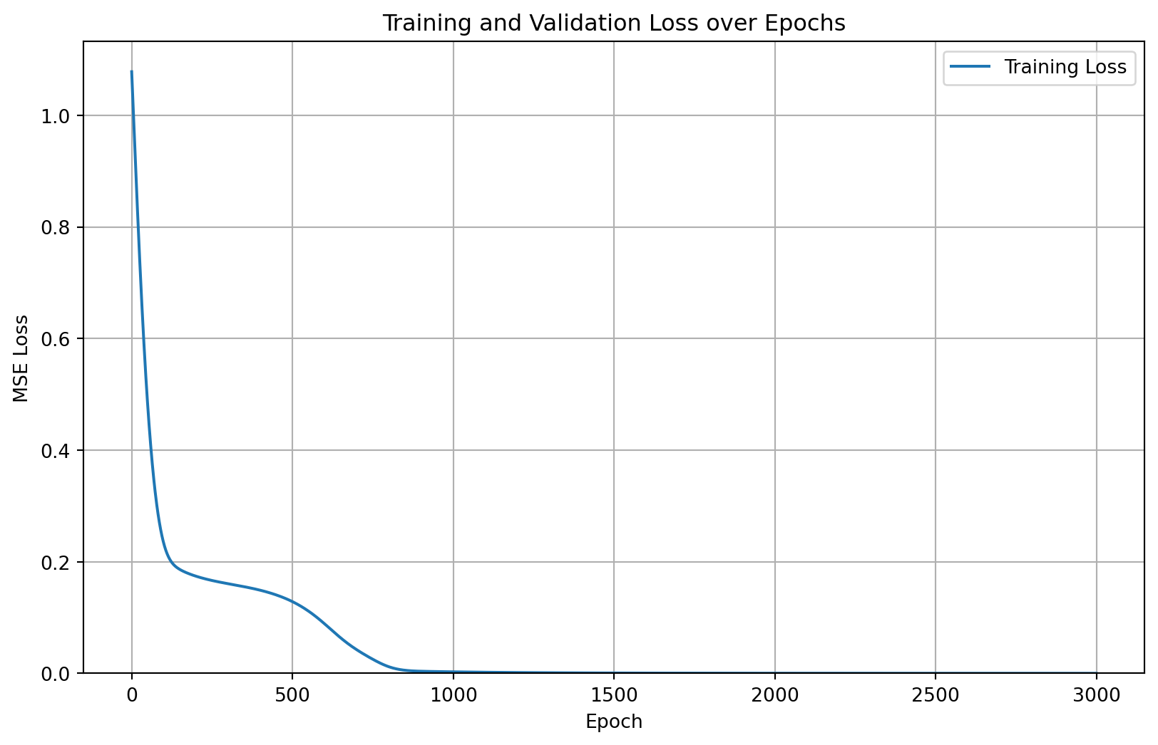
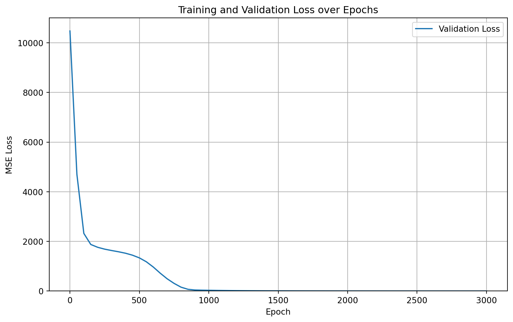
The following two plots show the training and validation loss curves. These provide a visual indication of how well the model is learning and whether it’s overfitting (which would be indicated by the training loss continuing to decrease while the validation loss starts to increase). In my case, the training loss closely follows the validation loss, suggesting that I likely reached a global minimum.

plt.figure(figsize=(10, 6))
plt.plot(train_losses, label="Training Loss")
# plt.plot(range(0,NUM_EPOCHS,50), [x for x in test_losses if x is not None], label="Validation Loss") #plot only not none values
plt.xlabel("Epoch")
plt.ylabel("MSE Loss")
plt.ylim(0, max(train_losses)*1.05)
plt.title("Training and Validation Loss over Epochs")
plt.legend()
plt.grid(True)
plt.show()


plt.figure(figsize=(10, 6))
# plt.plot(train_losses, label="Training Loss")
plt.plot(range(0,NUM_EPOCHS+1,50), [x for x in test_losses if x is not None][0:len(range(0,NUM_EPOCHS+1,50))], label="Validation Loss") #plot only not none values
plt.xlabel("Epoch")
plt.ylabel("MSE Loss")
plt.title("Training and Validation Loss over Epochs")
plt.ylim(0, max([x for x in test_losses if x is not None])*1.05)
plt.legend()
plt.grid(True)
plt.show()

Training and Validation Loss

It’s important to note that if the model had overfit the data, then the weight analysis would have been nearly useless.

5 Weight Evolution Analysis

This is the core of my analysis. I examine how the model’s weights change over the course of training. Because my GRU has a small number of parameters, I can visualize this evolution effectively. The PyTorch documentation helps us understand the names of the involved parameters:

• weight_ih_l[k] - the learnable input-hidden weights of the \(k^{th}\) layer (\(W_{ir}\)|\(W_{iz}\)|\(W_{in}\)), of shape \((3 * \text{hidden\_size}, \text{input\_size})\) for \(k=0\). In my example, with \(\text{hidden\_size} = 1\) and \(\text{input\_size} = 2\), this is \((3*1, 2)\), or \((3, 2)\).

• weight_hh_l[k] - the learnable hidden-hidden weights of the \(k^{th}\) layer (\(W_{hr}\)|\(W_{hz}\)|\(W_{hn}\)), of shape \((3 * \text{hidden\_size}, \text{hidden\_size})\). In my example, with \(\text{hidden\_size} = 1\), this is \((3*1, 1)\), or \((3, 1)\).

• bias_ih_l[k] - the learnable input-hidden bias of the \(k^{th}\) layer (\(b_{ir}\)|\(b_{iz}\)|\(b_{in}\)), of shape \((3 * \text{hidden\_size})\). In my example, with \(\text{hidden\_size} = 1\), this is \((3*1)\), or \((3)\).

• bias_hh_l[k] - the learnable hidden-hidden bias of the \(k^{th}\) layer (\(b_{hr}\)|\(b_{hz}\)|\(b_{hn}\)), of shape \((3 * \text{hidden\_size})\). In my example, with \(\text{hidden\_size} = 1\), this is \((3*1)\), or \((3)\).

I focused on the key weight matrices:

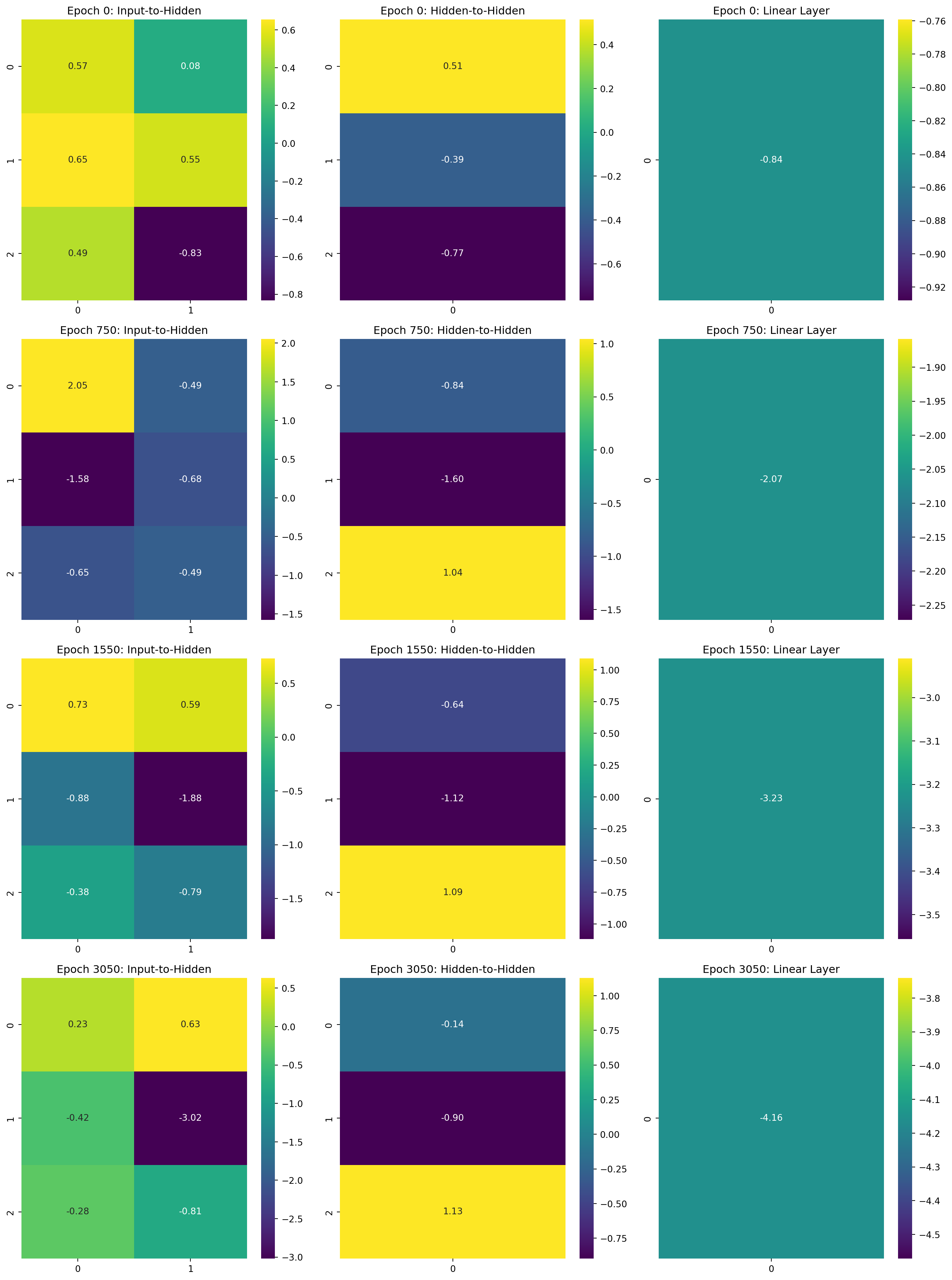
• gru.weight_ih_l0: Input-to-hidden weights. In my example, this has size \((3 \times 2)\).
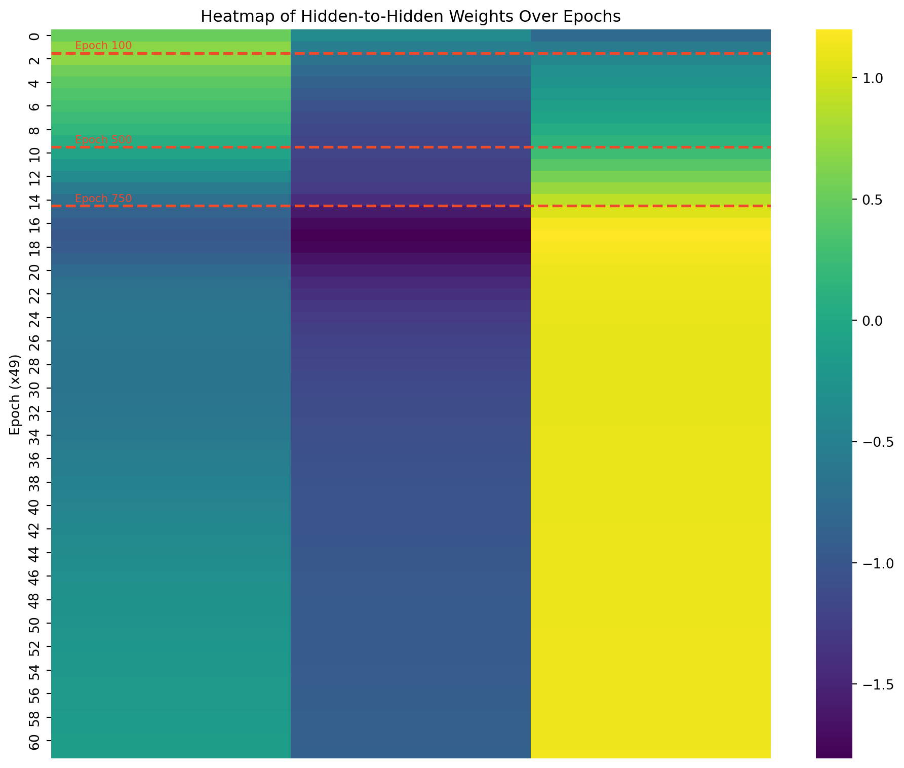
• gru.weight_hh_l0: Hidden-to-hidden weights. In my example, this has size \((3 \times 1)\).
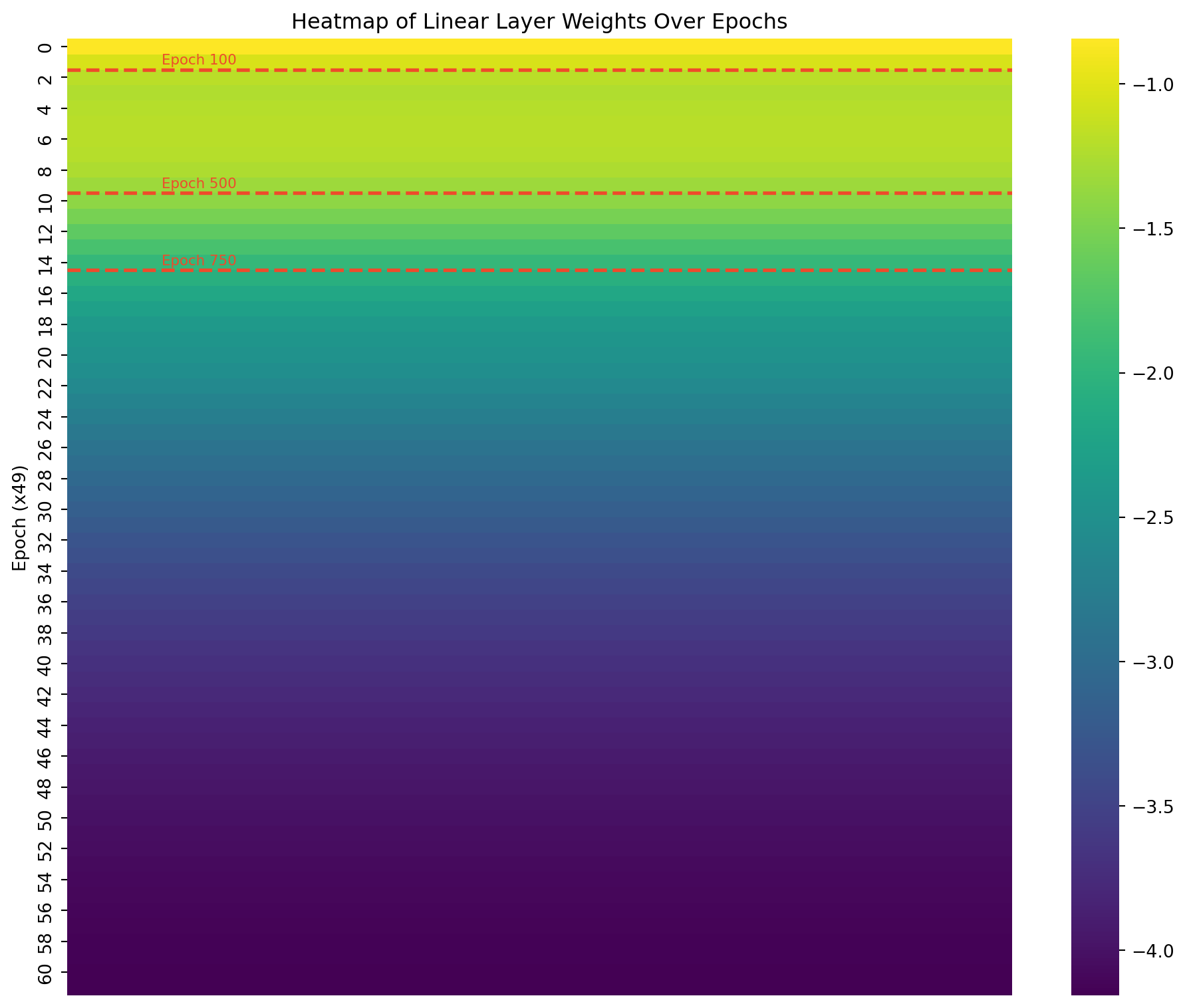
• linear.weight: Weights of the final linear layer. In my example, with \(\text{hidden\_size} = 1\) and \(\text{output\_size} = 1\), this has size \((1 \times 1)\). I included this to allow for potentially adding an additional dimension to the hidden layer later.

Now, here’s how GRUs work (it might look a little intimidating at first, but it’s actually quite straightforward):

Initially, for \(t = 0\), the output vector is \(h_0 = 0\).

\[\begin{aligned} z_t &= \sigma(W_z x_t + U_z h_{t-1} + b_z) \\ r_t &= \sigma(W_r x_t + U_r h_{t-1} + b_r) \\ \hat{h}_t &= \phi(W_h x_t + U_h (r_t \odot h_{t-1}) + b_h) \\ h_t &= (1 - z_t) \odot h_{t-1} + z_t \odot \hat{h}_t \end{aligned}\]

The \(W_{*}\) weights are the first set of weights (i.e., gru.weight_ih_l0), while the \(U_{*}\) weights are the second set of weights (i.e., gru.weight_hh_l0). The bias terms are straightforward, so I won’t go into detail.

I created plots showing the values of these weights at different stages of training. This visualization helps understand how the GRU learns to solve the adding problem. I used a heatmap to represent the weight matrices, making it easy to spot patterns and changes.

# Select a subset of epochs for clearer visualization
epochs_to_plot = [0, len(all_weights) // 4, len(all_weights) // 2, len(all_weights) - 1]
selected_weights = [all_weights[i] for i in epochs_to_plot]

# Plotting function for a single weight matrix
def plot_weight_matrix(weight_matrix, title, ax):
    sns.heatmap(weight_matrix, annot=True, fmt=".2f", cmap="viridis", cbar=True, ax=ax)
    ax.set_title(title)

fig, axes = plt.subplots(len(selected_weights), 3, figsize=(15, 5 * len(selected_weights)))

for i, epoch_weights in enumerate(selected_weights):
  plot_weight_matrix(epoch_weights['gru.weight_ih_l0'], f'Epoch {epochs_to_plot[i]*50}: Input-to-Hidden', axes[i, 0])
  plot_weight_matrix(epoch_weights['gru.weight_hh_l0'], f'Epoch {epochs_to_plot[i]*50}: Hidden-to-Hidden', axes[i, 1])
  plot_weight_matrix(epoch_weights['linear.weight'], f'Epoch {epochs_to_plot[i]*50}: Linear Layer', axes[i, 2])


plt.tight_layout()
plt.show()

Evolution of GRU + Linear Weights

6 Weight Dynamics and Learned Strategy

This section combines the detailed weight evolution visualizations (heatmaps and line plots) with the analysis of the GRU’s learned strategy. This provides a single, cohesive narrative.

import matplotlib.pyplot as plt
import seaborn as sns
import numpy as np

# Assuming all_weights is already loaded

weight_types = ['gru.weight_ih_l0', 'gru.weight_hh_l0', 'linear.weight']
weight_type_names = ['Input-to-Hidden', 'Hidden-to-Hidden', 'Linear Layer']

for i, weight_type in enumerate(weight_types):
    evolution_data = []
    for epoch_weights in all_weights:
        weight_matrix = epoch_weights[weight_type]
        if weight_type == 'gru.weight_ih_l0':
            evolution_data.append(weight_matrix.flatten(order='F'))
        else:
            evolution_data.append(weight_matrix.flatten())

    evolution_heatmap_data = np.array(evolution_data)

    fig, ax = plt.subplots(figsize=(10, 8))
    sns.heatmap(evolution_heatmap_data, cmap="viridis", cbar=True, ax=ax, xticklabels=False)

    ax.set_title(f'Heatmap of {weight_type_names[i]} Weights Over Epochs')
    ax.set_ylabel('Epoch (x49)')

    ax.axhline(2, color='#EE4B2B', linestyle='--', linewidth=2)
    ax.axhline(10, color='#EE4B2B', linestyle='--', linewidth=2)
    ax.axhline(15, color='#EE4B2B', linestyle='--', linewidth=2)


    if weight_type == 'gru.weight_ih_l0':
        ax.axvline(3, color='#EE4B2B')
        ax.text(x=0.1, y=60, s="Input[0]", color='#EE4B2B', fontsize=8,
            ha='left', va='bottom', bbox=dict(facecolor='black', alpha=0.3))
        ax.text(x=3.1, y=60, s="Input[1]", color='#EE4B2B', fontsize=8,
                ha='left', va='bottom', bbox=dict(facecolor='black', alpha=0.3))



    ax.text(x=0.1, y=2-.2, s="Epoch 100", color='#EE4B2B', fontsize=8,
        ha='left', va='bottom')
    ax.text(x=0.1, y=10-.2, s="Epoch 500", color='#EE4B2B', fontsize=8,
            ha='left', va='bottom')
    ax.text(x=0.1, y=15-.2, s="Epoch 750", color='#EE4B2B', fontsize=8,
        ha='left', va='bottom')


    plt.tight_layout()
    plt.show()

Combined Heatmap of Weight Evolution Over Epochs

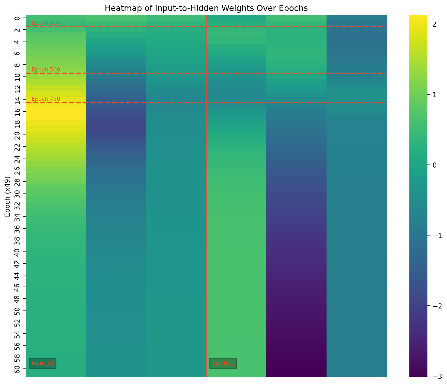
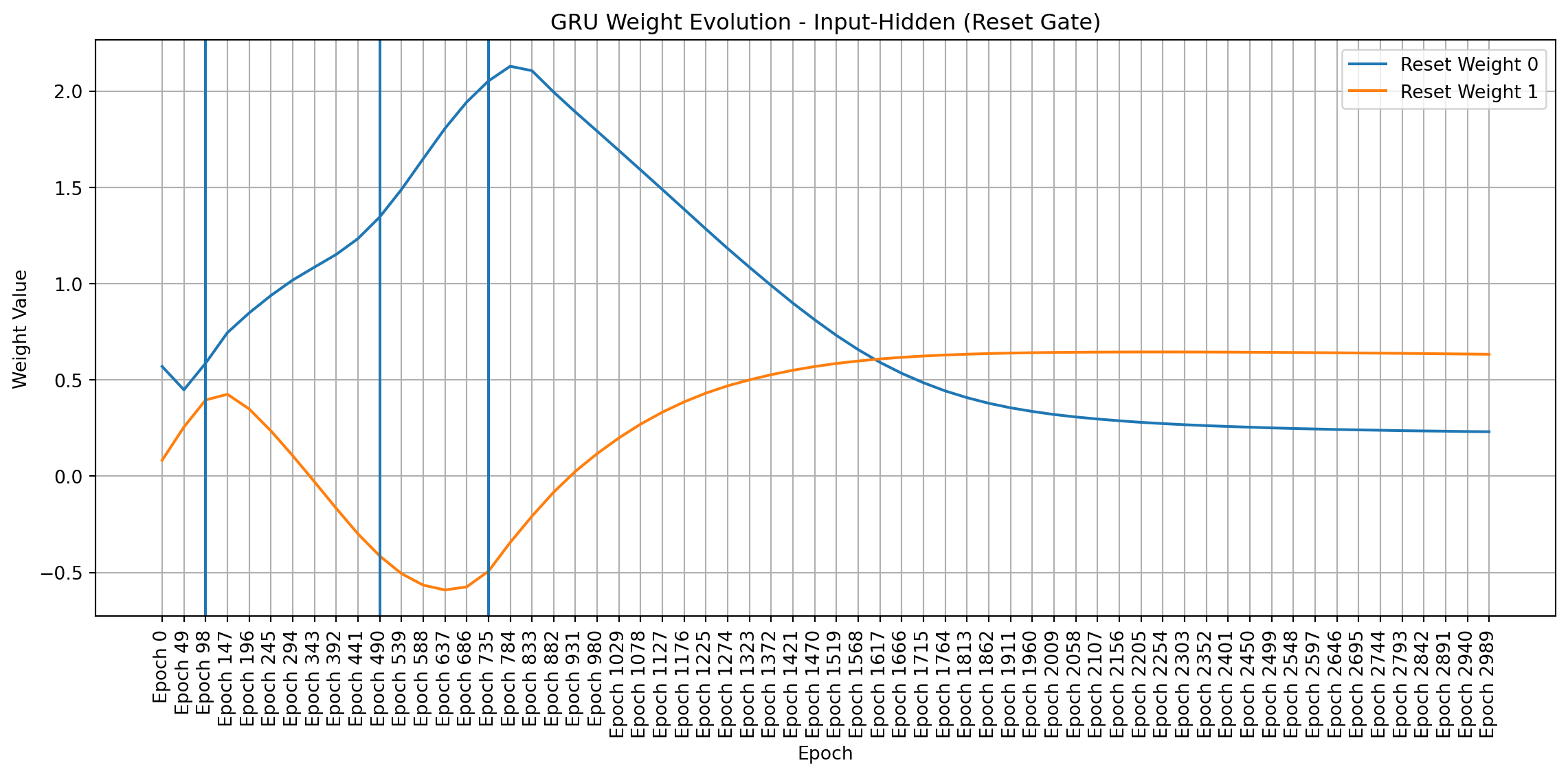
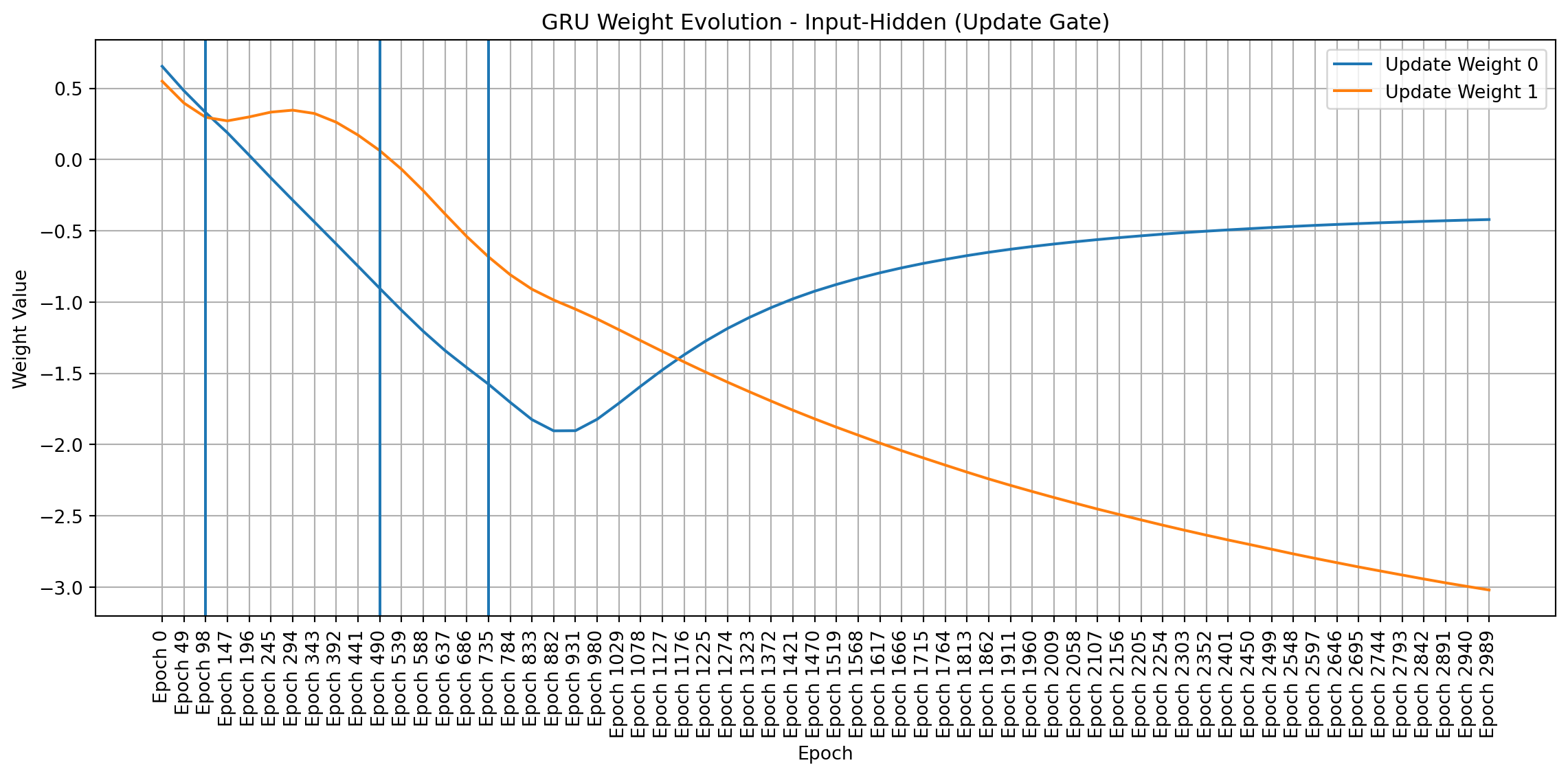
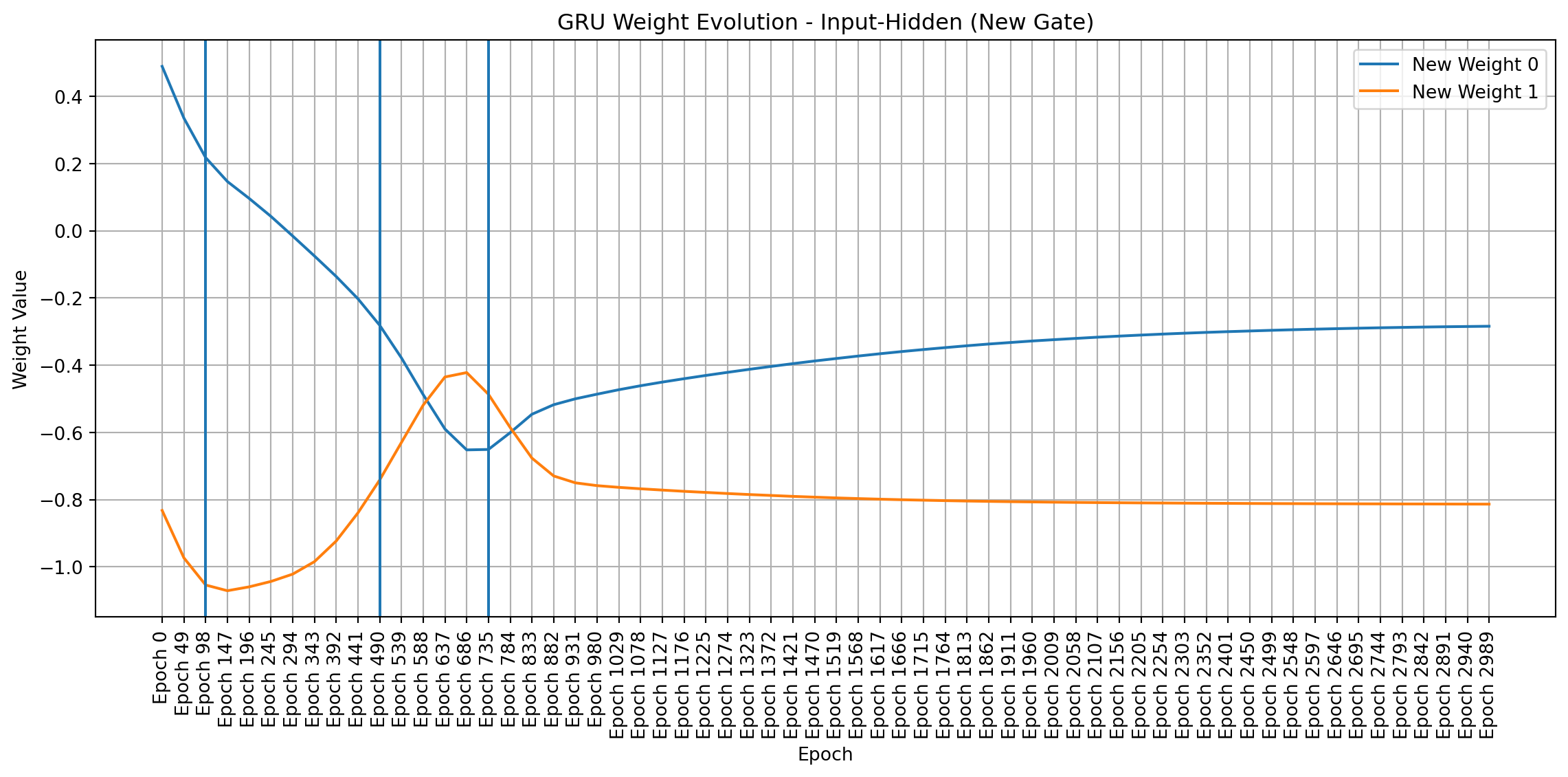
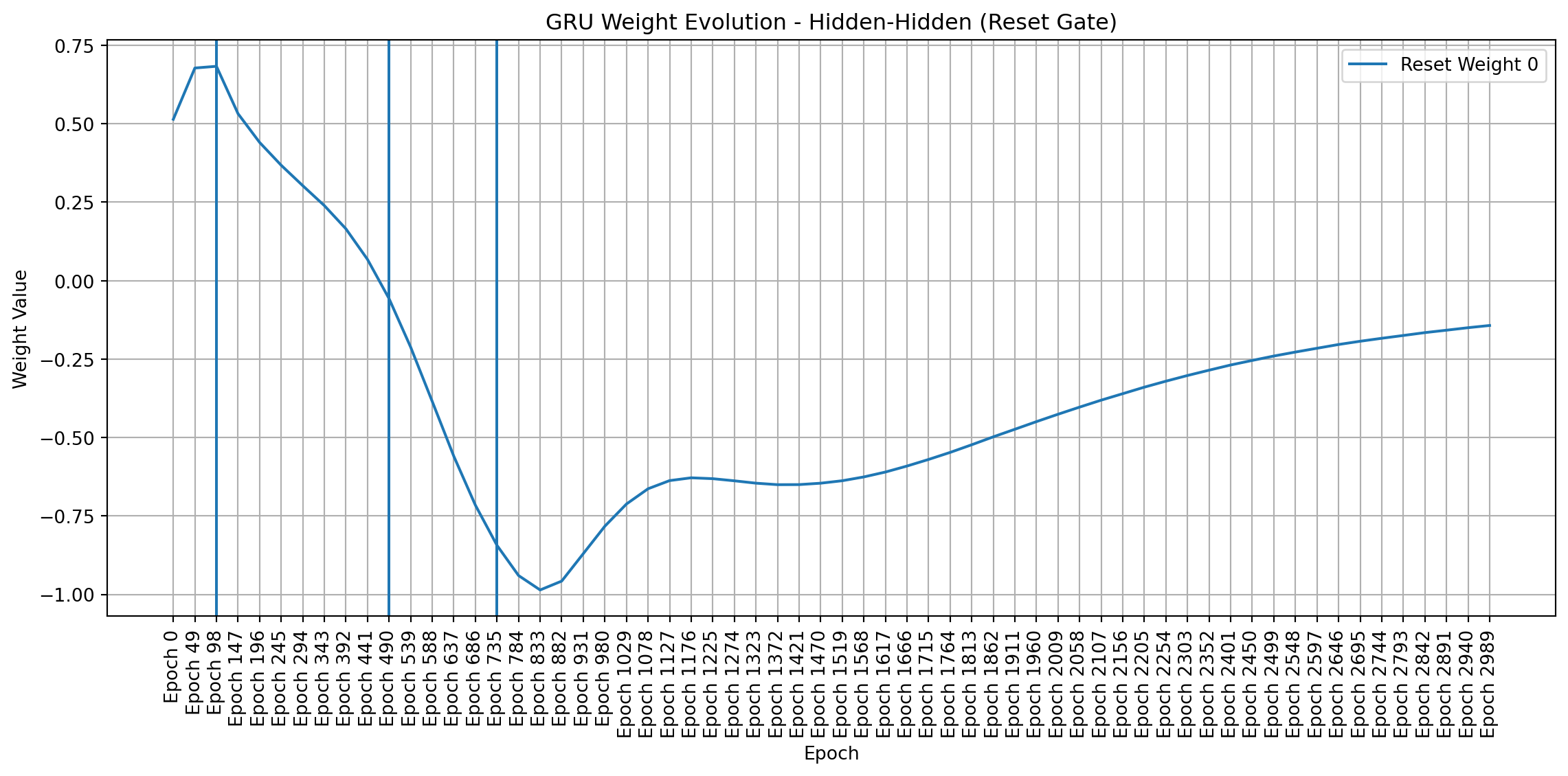
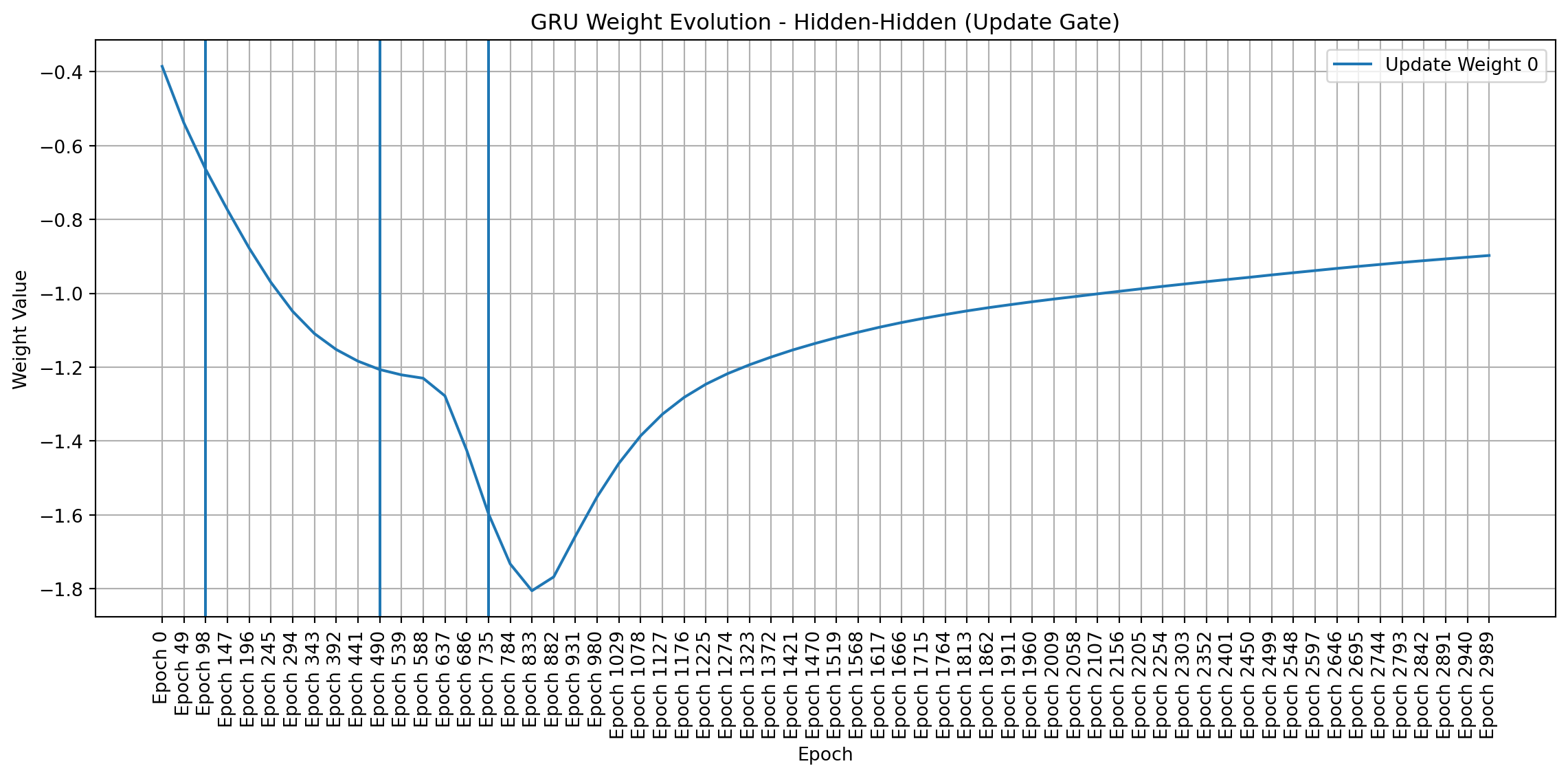
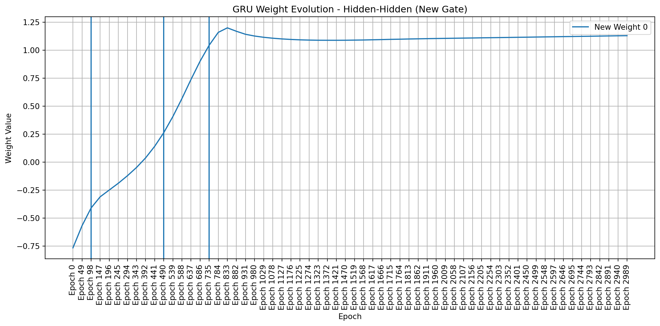
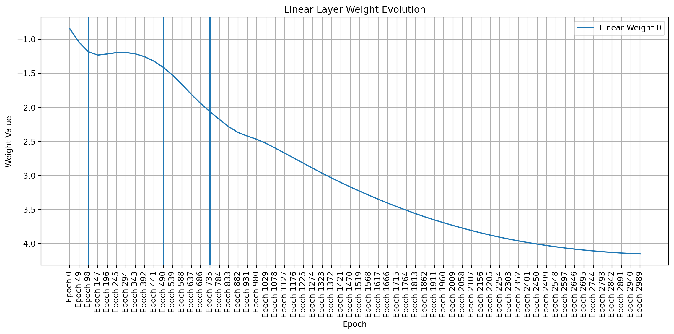
To visualize weight changes directly, I used line plots to show the evolution of individual weights across sampled epochs. These plots complement the heatmaps by providing a more detailed view of how each weight changes in magnitude and direction. Plotting signed values reveals symmetries and patterns that emerge during training, even in a simple network like mine.

import matplotlib.pyplot as plt
import pandas as pd
import numpy as np  # Make sure numpy is imported

def plot_gru_weight_evolution(all_weights, title_prefix):
    """
    Plots the evolution of GRU weight matrices (input-hidden, hidden-hidden)
    separated by gate (Reset, Update, New).
    """

    def plot_single_gate_weights(weight_values, gate_name, title):
        """Helper function to plot weights for a single gate."""
        df = pd.DataFrame(weight_values).T
        df.columns = [f"Epoch {i*49}" for i in range(len(all_weights))]

        plt.figure(figsize=(12, 6))
        for i in range(df.shape[0]):
            plt.plot(df.columns, df.iloc[i], label=f"{gate_name} Weight {i}")  # Add weight index to label

        plt.title(title)
        plt.xlabel("Epoch")
        plt.ylabel("Weight Value")
        plt.xticks(rotation=90)
        plt.legend()
        plt.grid(True)
        plt.axvline(x="Epoch 98")
        plt.axvline(x="Epoch 490")
        plt.axvline(x="Epoch 735")
        plt.tight_layout()
        plt.show()

    # --- Input-to-Hidden Weights ---
    ih_weights = [all_weights[i]["gru.weight_ih_l0"] for i in range(len(all_weights))]
    # Split into Reset, Update, and New gate weights (assuming standard GRU structure)
    ih_reset_weights = [w[0:w.shape[0]//3, :].flatten() for w in ih_weights]
    ih_update_weights = [w[w.shape[0]//3:2*w.shape[0]//3, :].flatten() for w in ih_weights]
    ih_new_weights = [w[2*w.shape[0]//3:, :].flatten() for w in ih_weights]

    plot_single_gate_weights(ih_reset_weights, "Reset", f"{title_prefix} - Input-Hidden (Reset Gate)")
    plot_single_gate_weights(ih_update_weights, "Update", f"{title_prefix} - Input-Hidden (Update Gate)")
    plot_single_gate_weights(ih_new_weights, "New", f"{title_prefix} - Input-Hidden (New Gate)")

    # --- Hidden-to-Hidden Weights ---
    hh_weights = [all_weights[i]["gru.weight_hh_l0"] for i in range(len(all_weights))]
    # Split into Reset, Update, and New gate weights
    hh_reset_weights = [w[0:w.shape[0]//3, :].flatten() for w in hh_weights]
    hh_update_weights = [w[w.shape[0]//3:2*w.shape[0]//3, :].flatten() for w in hh_weights]
    hh_new_weights = [w[2*w.shape[0]//3:, :].flatten() for w in hh_weights]

    plot_single_gate_weights(hh_reset_weights, "Reset", f"{title_prefix} - Hidden-Hidden (Reset Gate)")
    plot_single_gate_weights(hh_update_weights, "Update", f"{title_prefix} - Hidden-Hidden (Update Gate)")
    plot_single_gate_weights(hh_new_weights, "New", f"{title_prefix} - Hidden-Hidden (New Gate)")



def plot_linear_weight_evolution(all_weights, title):
    """Plots the evolution of the linear layer weights."""
    weight_values = [all_weights[i]["linear.weight"].flatten() for i in range(len(all_weights))]

    df = pd.DataFrame(weight_values).T
    df.columns = [f"Epoch {i*49}" for i in range(len(all_weights))]

    plt.figure(figsize=(12, 6))
    for i in range(df.shape[0]):
        plt.plot(df.columns, df.iloc[i], label=f"Linear Weight {i}")

    plt.title(title)
    plt.xlabel("Epoch")
    plt.ylabel("Weight Value")
    plt.xticks(rotation=90)
    plt.legend()
    plt.grid(True)
    plt.axvline(x="Epoch 98")
    plt.axvline(x="Epoch 490")
    plt.axvline(x="Epoch 735")
    plt.tight_layout()
    plt.show()


# Create the plots
plot_gru_weight_evolution(all_weights, "GRU Weight Evolution")
plot_linear_weight_evolution(all_weights, "Linear Layer Weight Evolution")

Weight Dynamics Over Training

7 Illustrative Example: Forward Pass

To further clarify how the trained GRU operates, I’ll walk through a single forward pass with a concrete example. This will demonstrate the roles of the input-to-hidden weights, hidden-to-hidden weights, and the final linear layer, as well as how the binary mask selects the relevant input values.

Example Input:

The input sequence is represented as a tensor:

\[ \text{input\_sequence} = \begin{bmatrix} 12 & 0 \\ 37 & 1 \\ 12 & 0 \\ 21 & 1 \end{bmatrix} \]

The problem requires summing the values in the first dimension (column) only when the corresponding value in the second dimension (column) is 1 (the flag). In this example:

• The second element, \([37, 1]\), has a flag of 1, so 37 is included in the sum.
• The fourth element, \([21, 1]\), has a flag of 1, so 21 is included in the sum.
• The first and third elements have flags of 0, so their first-dimension values (12 and 12) are excluded.

Therefore, the expected output is \(37 + 21 = 58\).

input_sequence = torch.tensor([
    [12,0],
    [37,1],
    [12,0],
    [21,1],
]).float().unsqueeze(0)


input_sequence[:, :, 0] /= HIGH

And a quick sanity check applying my model. The result is: \(57.80980587005615\approx58\)

which is really close to the actual sum (\(37 + 21 = 58\))!!!!

Loaded Weights (from the last training epoch):

I used the weights from the last epoch of training, which I previously saved. This ensures that I’m using the fully trained model. Let’s get the weights:

# Get weights from the last training epoch.  'all_weights' is populated by the loading/training section.
last_epoch_weights = model.state_dict() #all_weights[-1]

# Extract the relevant weight matrices
W_ih = torch.tensor(last_epoch_weights['gru.weight_ih_l0']).float()  # Input-to-hidden
W_hh = torch.tensor(last_epoch_weights['gru.weight_hh_l0']).float()  # Hidden-to-hidden
b_ih = torch.tensor(last_epoch_weights['gru.bias_ih_l0']).float()  # Input-to-hidden bias
b_hh = torch.tensor(last_epoch_weights['gru.bias_hh_l0']).float()  # Hidden-to-hidden bias
W_linear = torch.tensor(last_epoch_weights['linear.weight']).float() # Linear layer weights
b_linear = torch.tensor(last_epoch_weights['linear.bias']).float()   # Linear layer bias

Now, let’s walk through the GRU step-by-step for each element in our input sequence.

For each element, I calculate the Update Gate (\(z_t\)), Reset Gate (\(r_t\)), New Gate (\(\tilde{h}_t\)), and Hidden State (\(h_t\)).

I start by initializing the hidden state to zero:

h_t = torch.zeros(1, 1, 1) # Initialize hidden state

\[ h_t = 0.0 \]

7.1 Step 1: Input \([12, 0]\)

Input for Step 1: \[ x_1 = \begin{bmatrix} 0.12 & 0 \end{bmatrix} \]

1. Update Gate \(z_1\): \[ z_1 = \sigma(x_1 W_{iz}^T + h_0 W_{hz}^T + b_{iz}) \]

   x_1 = input_sequence[:, 0, :]
   h = torch.zeros(1, 1, 1)
   
   # Stable version (using torch.matmul)
   gi_stable = torch.matmul(x_1, W_ih.t()) + b_ih
   gh_stable = torch.matmul(h, W_hh.t()) + b_hh
   
   # Get gates
   i_r, i_z, i_n = gi_stable.chunk(3, dim=1)
   h_r, h_z, h_n = gh_stable.chunk(3, dim=2)
   
   # Apply gate operations with controlled precision
   resetgate = torch.sigmoid(i_r + h_r)
   updategate = torch.sigmoid(i_z + h_z)
   newgate = torch.tanh(i_n + (resetgate * h_n))
   
   hy = (1 - updategate) * newgate + updategate * h
   h_t = hy

   Update Gate: \[ z_1 = 0.8275274634361267 \]

2. Reset Gate \(r_1\): \[ r_1 = \sigma(x_1 W_{ir}^T + h_0 W_{hr}^T + b_{ir}) \]

   Reset Gate: \[ r_1 = 0.819507896900177 \]

3. New Gate \(\tilde{h}_1\): \[ \tilde{h}_1 = \tanh(x_1 W_{in}^T + (r_1 \odot h_0) W_{hn}^T + b_{in}) \]

   New Gate: \[ \tilde{h}_1 = 0.639545738697052 \]

4. Hidden State \(h_1\): \[ h_1 = (1 - z_1) \odot h_0 + z_1 \odot \tilde{h}_1 \]

   Hidden State: \[ h_1 = 0.11030407249927521 \]

7.2 Step 2: Input \([37, 1]\)

Input for Step 2: \[ x_2 = \begin{bmatrix} 0.37 & 1 \end{bmatrix} \]

1. Update Gate \(z_2\): \[ z_2 = \sigma(x_2 W_{iz}^T + h_1 W_{hz}^T + b_{iz}) \]

   x_2 = input_sequence[:, 1, :]
   
   # Stable version (using torch.matmul)
   gi_stable = torch.matmul(x_2, W_ih.t()) + b_ih
   gh_stable = torch.matmul(h_t, W_hh.t()) + b_hh
   
   # Get gates
   i_r, i_z, i_n = gi_stable.chunk(3, dim=1)
   h_r, h_z, h_n = gh_stable.chunk(3, dim=2)
   
   # Apply gate operations
   resetgate2 = torch.sigmoid(i_r + h_r)
   updategate2 = torch.sigmoid(i_z + h_z)
   newgate2 = torch.tanh(i_n + (resetgate2 * h_n))
   
   hy = (1 - updategate2) * newgate2 + updategate2 * h_t
   h_t = hy

   Update Gate: \[ z_2 = 0.15969596803188324 \]

2. Reset Gate \(r_2\): \[ r_2 = \sigma(x_2 W_{ir}^T + h_1 W_{hr}^T + b_{ir}) \]

   Reset Gate: \[ r_2 = 0.89918053150177 \]

3. New Gate \(\tilde{h}_2\): \[ \tilde{h}_2 = \tanh(x_2 W_{in}^T + (r_2 \odot h_1) W_{hn}^T + b_{in}) \]

   New Gate: \[ \tilde{h}_2 = -0.001833615591749549 \]

4. Hidden State \(h_2\): \[ h_2 = (1 - z_2) \odot h_1 + z_2 \odot \tilde{h}_2 \]

   Hidden State: \[ h_2 = 0.016074320301413536 \]

7.3 Step 3: Input \([12, 0]\)

Input for Step 3: \[ x_3 = \begin{bmatrix} 0.12 & 0 \end{bmatrix} \]

1. Update Gate \(z_3\): \[ z_3 = \sigma(x_3 W_{iz}^T + h_2 W_{hz}^T + b_{iz}) \]

   x_3 = input_sequence[:, 2, :]
   
   # Stable version (using torch.matmul)
   gi_stable = torch.matmul(x_3, W_ih.t()) + b_ih
   gh_stable = torch.matmul(h_t, W_hh.t()) + b_hh
   
   # Get gates
   i_r, i_z, i_n = gi_stable.chunk(3, dim=1)
   h_r, h_z, h_n = gh_stable.chunk(3, dim=2)
   
   # Apply gate operations
   resetgate3 = torch.sigmoid(i_r + h_r)
   updategate3 = torch.sigmoid(i_z + h_z)
   newgate3 = torch.tanh(i_n + (resetgate3 * h_n))
   
   hy = (1 - updategate3) * newgate3 + updategate3 * h_t
   h_t = hy

   Update Gate: \[ z_3 = 0.8254608511924744 \]

2. Reset Gate \(r_3\): \[ r_3 = \sigma(x_3 W_{ir}^T + h_2 W_{hr}^T + b_{ir}) \]

   Reset Gate: \[ r_3 = 0.8191711902618408 \]

3. New Gate \(\tilde{h}_3\): \[ \tilde{h}_3 = \tanh(x_3 W_{in}^T + (r_3 \odot h_2) W_{hn}^T + b_{in}) \]

   New Gate: \[ \tilde{h}_3 = 0.648215115070343 \]

4. Hidden State \(h_3\): \[ h_3 = (1 - z_3) \odot h_2 + z_3 \odot \tilde{h}_3 \]

   Hidden State: \[ h_3 = 0.12640763819217682 \]

7.4 Step 4: Input \([21, 1]\)

Input for Step 4: \[ x_4 = \begin{bmatrix} 0.21 & 1 \end{bmatrix} \]

1. Update Gate \(z_4\): \[ z_4 = \sigma(x_4 W_{iz}^T + h_3 W_{hz}^T + b_{iz}) \]

   x_4 = input_sequence[:, 3, :]
   
   
   # Stable version (using torch.matmul)
   gi_stable = torch.matmul(x_4, W_ih.t()) + b_ih
   gh_stable = torch.matmul(h_t, W_hh.t()) + b_hh
   
   # Get gates
   i_r, i_z, i_n = gi_stable.chunk(3, dim=1)
   h_r, h_z, h_n = gh_stable.chunk(3, dim=2)
   
   # Apply gate operations
   resetgate4 = torch.sigmoid(i_r + h_r)
   updategate4 = torch.sigmoid(i_z + h_z)
   newgate4 = torch.tanh(i_n + (resetgate4 * h_n))
   
   hy = (1 - updategate4) * newgate4 + updategate4 * h_t
   h_t = hy

   Update Gate: \[ z_4 = 0.1668987274169922 \]

2. Reset Gate \(r_4\): \[ r_4 = \sigma(x_4 W_{ir}^T + h_3 W_{hr}^T + b_{ir}) \]

   Reset Gate: \[ r_4 = 0.8955692052841187 \]

3. New Gate \(\tilde{h}_4\): \[ \tilde{h}_4 = \tanh(x_4 W_{in}^T + (r_4 \odot h_3) W_{hn}^T + b_{in}) \]

   New Gate: \[ \tilde{h}_4 = 0.05876209959387779 \]

4. Hidden State \(h_4\): \[ h_4 = (1 - z_4) \odot h_3 + z_4 \odot \tilde{h}_4 \]

   Hidden State: \[ h_4 = 0.07005205750465393 \]

7.5 Step 5: Linear Layer

Finally, the hidden state \(h_4\) is passed through the linear layer to produce the output.

\[ \text{output} = h_4 W_{\text{linear}}^T + b_{\text{linear}} \]

output = h_t @ W_linear.T + b_linear

Linear Layer output: \[ \text{output} = 57.8097939491272 \]

The final result, as we can see, when approximated using the ceiling function, matches the expected result of 58.

8 Coming next…

This post set some ground work for a more thorough analysis of the model’s weights. I’ve trained a simple model, and now it’s time to crack it open and see what makes it tick. Think of it like this: usually these models are black boxes, and the weights that are inside and make them move or somwhat foggy to us. I’m going to be taking a close look at what those gears and levers look like after all the training is done – are they big or small? Are they organized in any particular way? What do they do?

But it’s not enough just to look at them. I want to figure out what they actually do. Each weight contributes, in some way, to the final output of the model. I’ll be exploring how different weights, or groups of weights, affect the model’s predictions. I might even try tweaking them a bit to see what happens! This is like figuring out which lever controls which part of the machine.

And finally, the really fun part: I’ll try to guess how they got that way. The training process is like a long and winding road, and the weights are constantly changing along the way. I’ll try to reconstruct that journey, piecing together clues from the final weights to understand the path the model took to learn. It’s a bit like detective work, trying to figure out the story behind the final result and I just love that! Get ready for some serious model investigation!