1 Introduction

In Part 3, we discovered something fascinating: our GRU with a hidden size of 1 couldn’t solve the general adding problem, not because of insufficient storage space, but because of the fundamental mathematical constraints of smooth activation functions trying to perform discrete information operations. Basically the architecture of a GRU performs a continuous transformation of the input data, which is not suitable for tasks that require precise bitwise operations, or in general discrete information manipulation.

This raised a profound question that deserves a blog post in its own right: How much information can a single neural network cell actually contain, and what are the theoretical limits imposed by activation functions like sigmoid and tanh? Can we in principle give a precise upper bound on this capacity? And can we set up a theoretical framework to calculate it based on the activation functions used, the dimensions and the overall architecture?

In this bonus section, we’ll conduct a series of targeted experiments to:

Measure the practical information capacity of a single GRU cell across different tasks
Quantify how activation functions limit information encoding capabilities
Explore the trade-off between smooth interpolation and discrete logic
Validate our information bottleneck theory with controlled experiments
Compare theoretical Shannon entropy limits with empirical performance

This is just academic curiosity—understanding, not solving the adding problem. Having an answer to these question could help me design a better architecture in the future when I start working on my actual main project which is a neural network that can play connect 4 with the smallest possible architecture.

Note for fast preview: To preview this document quickly without training models, run:

SKIP_TRAINING=1 quarto preview projects/adding-problem-part3-5.qmd

Let’s dive in!

2 Experiment 1: Information Capacity Measurement

Our first experiment directly measures how many bits of information a single GRU cell can reliably encode and retrieve. We’ll start simple and progressively increase complexity until we hit the ceiling.

Code

import torch
import torch.nn as nn
import torch.nn.functional as F
import numpy as np
import matplotlib.pyplot as plt
import seaborn as sns
from torch.utils.data import DataLoader, TensorDataset
from tqdm.notebook import trange, tqdm
import pandas as pd
from sklearn.metrics import accuracy_score
import json
import os

# Global flag to skip training during preview (set to True for fast preview)
# Can be controlled via environment variable: export SKIP_TRAINING=1
SKIP_TRAINING = os.environ.get('SKIP_TRAINING', 'false').lower() in ['true', '1', 'yes']

# Reproducibility
RANDOM_SEED = 42
np.random.seed(RANDOM_SEED)
torch.manual_seed(RANDOM_SEED)

class SingleCellGRU(nn.Module):
    """GRU with exactly 1 hidden unit for measuring information capacity"""
    def __init__(self, input_size, num_classes, activation='tanh'):
        super(SingleCellGRU, self).__init__()
        self.gru = nn.GRU(input_size, 1, num_layers=1, batch_first=True)
        self.classifier = nn.Linear(1, num_classes)
        self.activation = activation
        
        # Override activation if needed
        if activation == 'relu':
            # Replace tanh with ReLU in GRU (hack)
            self.gru.activation = torch.relu
        
    def forward(self, x):
        out, hn = self.gru(x)
        # Use final hidden state for classification
        output = self.classifier(hn.squeeze(0))
        return output

def generate_classification_data(n_samples, seq_len, num_classes, task_type='random'):
    """Generate classification tasks of varying complexity"""
    
    if task_type == 'random':
        # Pure random classification - maximum entropy
        X = torch.randn(n_samples, seq_len, 1)
        y = torch.randint(0, num_classes, (n_samples,))
        
    elif task_type == 'pattern_sum':
        # Classification based on sum of sequence
        X = torch.randn(n_samples, seq_len, 1)
        sums = X.sum(dim=1).squeeze()
        # Divide sum range into num_classes bins
        percentiles = torch.quantile(sums, torch.linspace(0, 1, num_classes + 1))
        y = torch.searchsorted(percentiles[1:-1], sums).long()
        
    elif task_type == 'pattern_count':
        # Classification based on counting positive values
        X = torch.randn(n_samples, seq_len, 1)
        counts = (X > 0).sum(dim=1).squeeze()
        # Map counts to classes
        y = (counts % num_classes).long()
        
    elif task_type == 'pattern_last':
        # Classification based on last value only
        X = torch.randn(n_samples, seq_len, 1)
        last_vals = X[:, -1, 0]
        percentiles = torch.quantile(last_vals, torch.linspace(0, 1, num_classes + 1))
        y = torch.searchsorted(percentiles[1:-1], last_vals).long()
        
    return X, y

def train_and_evaluate(model, train_loader, test_loader, epochs=100, lr=0.001):
    """Train model and return final accuracy"""
    criterion = nn.CrossEntropyLoss()
    optimizer = torch.optim.Adam(model.parameters(), lr=lr)
    
    model.train()
    for epoch in range(epochs):
        for inputs, labels in train_loader:
            optimizer.zero_grad()
            outputs = model(inputs)
            loss = criterion(outputs, labels)
            loss.backward()
            optimizer.step()
    
    # Evaluate
    model.eval()
    all_preds = []
    all_labels = []
    
    with torch.no_grad():
        for inputs, labels in test_loader:
            outputs = model(inputs)
            preds = torch.argmax(outputs, dim=1)
            all_preds.extend(preds.cpu().numpy())
            all_labels.extend(labels.cpu().numpy())
    
    return accuracy_score(all_labels, all_preds)

# Run capacity measurement experiment
def measure_information_capacity():
    """Measure how many bits a single cell can handle across different tasks"""
    
    # Cache file for experiment 1
    cache_file = "experiment1_capacity_results.json"
    
    if SKIP_TRAINING:
        print("SKIP_TRAINING is True - returning placeholder data for experiment 1")
        # Create placeholder data for visualization
        placeholder_data = []
        for activation in ['tanh', 'relu']:
            for task_type in ['pattern_sum', 'pattern_count']:
                for bits in [1, 2, 3, 4]:
                    placeholder_data.append({
                        'activation': activation,
                        'task_type': task_type,
                        'num_classes': 2**bits,
                        'bits_required': bits,
                        'accuracy': max(0.5, 1 - bits*0.15) + np.random.random()*0.1,
                        'random_baseline': 1.0/(2**bits),
                        'above_random': bits <= 3
                    })
        return pd.DataFrame(placeholder_data)
    
    if os.path.exists(cache_file):
        print("Loading cached results from experiment 1...")
        with open(cache_file, 'r') as f:
            cached_data = json.load(f)
        return pd.DataFrame(cached_data)
    
    print("Running experiment 1 (this may take a while)...")
    results = []
    n_samples = 5000
    seq_len = 10
    train_split = 0.8
    
    # Test different numbers of classes (bits = log2(classes))
    class_counts = [2, 4, 8, 16, 32, 64, 128]  # 1 to 7 bits
    task_types = ['pattern_sum', 'pattern_count', 'pattern_last', 'random']
    activations = ['tanh', 'relu']
    
    for activation in activations:
        for task_type in task_types:
            for num_classes in class_counts:
                bits_required = np.log2(num_classes)
                
                # Generate data
                X, y = generate_classification_data(n_samples, seq_len, num_classes, task_type)
                
                # Split data
                train_size = int(train_split * n_samples)
                train_X, test_X = X[:train_size], X[train_size:]
                train_y, test_y = y[:train_size], y[train_size:]
                
                train_dataset = TensorDataset(train_X, train_y)
                test_dataset = TensorDataset(test_X, test_y)
                train_loader = DataLoader(train_dataset, batch_size=64, shuffle=True)
                test_loader = DataLoader(test_dataset, batch_size=64, shuffle=False)
                
                # Train model
                model = SingleCellGRU(1, num_classes, activation)
                accuracy = train_and_evaluate(model, train_loader, test_loader)
                
                # Random baseline
                random_baseline = 1.0 / num_classes
                
                results.append({
                    'activation': activation,
                    'task_type': task_type,
                    'num_classes': num_classes,
                    'bits_required': bits_required,
                    'accuracy': accuracy,
                    'random_baseline': random_baseline,
                    'above_random': accuracy > random_baseline * 1.1  # 10% margin
                })
                
                print(f"{activation} | {task_type} | {num_classes} classes ({bits_required:.1f} bits): {accuracy:.3f}")
    
    # Save results to cache
    with open(cache_file, 'w') as f:
        json.dump(results, f)
    
    return pd.DataFrame(results)

# Run the experiment
print("Measuring information capacity of single GRU cell...")
capacity_results = measure_information_capacity()

Measuring information capacity of single GRU cell...
Loading cached results from experiment 1...

Code

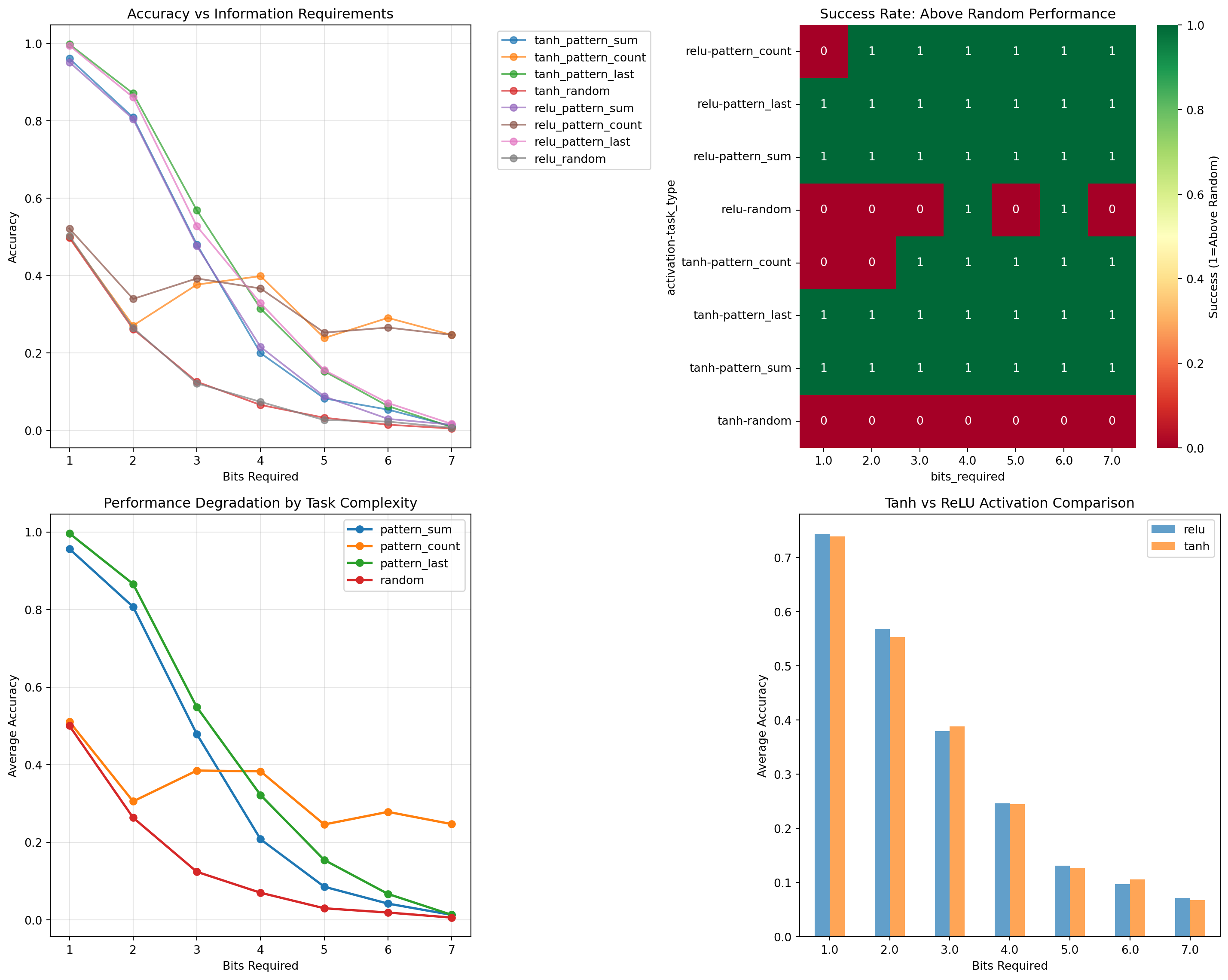
# Visualize results
fig, axes = plt.subplots(2, 2, figsize=(15, 12))

# Plot 1: Accuracy vs Bits Required (by activation)
for activation in capacity_results['activation'].unique():
    data = capacity_results[capacity_results['activation'] == activation]
    
    for task_type in data['task_type'].unique():
        task_data = data[data['task_type'] == task_type]
        axes[0, 0].plot(task_data['bits_required'], task_data['accuracy'], 
                       'o-', label=f'{activation}_{task_type}', alpha=0.7)

axes[0, 0].set_xlabel('Bits Required')
axes[0, 0].set_ylabel('Accuracy')
axes[0, 0].set_title('Accuracy vs Information Requirements')
axes[0, 0].legend(bbox_to_anchor=(1.05, 1), loc='upper left')
axes[0, 0].grid(True, alpha=0.3)

# Plot 2: Success rate (above random) heatmap
success_pivot = capacity_results.pivot_table(
    values='above_random', 
    index=['activation', 'task_type'], 
    columns='bits_required', 
    aggfunc='first'
).astype(int)

sns.heatmap(success_pivot, annot=True, cmap='RdYlGn', ax=axes[0, 1], 
            cbar_kws={'label': 'Success (1=Above Random)'})
axes[0, 1].set_title('Success Rate: Above Random Performance')

# Plot 3: Accuracy drop-off by task type
for task_type in capacity_results['task_type'].unique():
    task_data = capacity_results[capacity_results['task_type'] == task_type]
    grouped = task_data.groupby('bits_required')['accuracy'].mean()
    axes[1, 0].plot(grouped.index, grouped.values, 'o-', label=task_type, linewidth=2)

axes[1, 0].set_xlabel('Bits Required')
axes[1, 0].set_ylabel('Average Accuracy')
axes[1, 0].set_title('Performance Degradation by Task Complexity')
axes[1, 0].legend()
axes[1, 0].grid(True, alpha=0.3)

# Plot 4: Activation function comparison
activation_comparison = capacity_results.groupby(['activation', 'bits_required'])['accuracy'].mean().unstack(level=0)
activation_comparison.plot(kind='bar', ax=axes[1, 1], alpha=0.7)
axes[1, 1].set_xlabel('Bits Required')
axes[1, 1].set_ylabel('Average Accuracy')
axes[1, 1].set_title('Tanh vs ReLU Activation Comparison')
axes[1, 1].legend()
axes[1, 1].tick_params(axis='x', rotation=0)

plt.tight_layout()
plt.show()

# Find the capacity ceiling
print("\nCapacity Analysis:")
for activation in capacity_results['activation'].unique():
    act_data = capacity_results[capacity_results['activation'] == activation]
    successful_bits = act_data[act_data['above_random']]['bits_required']
    if len(successful_bits) > 0:
        max_bits = successful_bits.max()
        print(f"{activation}: Can handle up to {max_bits:.1f} bits reliably")
    else:
        print(f"{activation}: Cannot handle any classification tasks reliably")

# Experiment 2: Activation Function Limitations

Information Capacity Measurement Results


Capacity Analysis:
tanh: Can handle up to 7.0 bits reliably
relu: Can handle up to 7.0 bits reliably

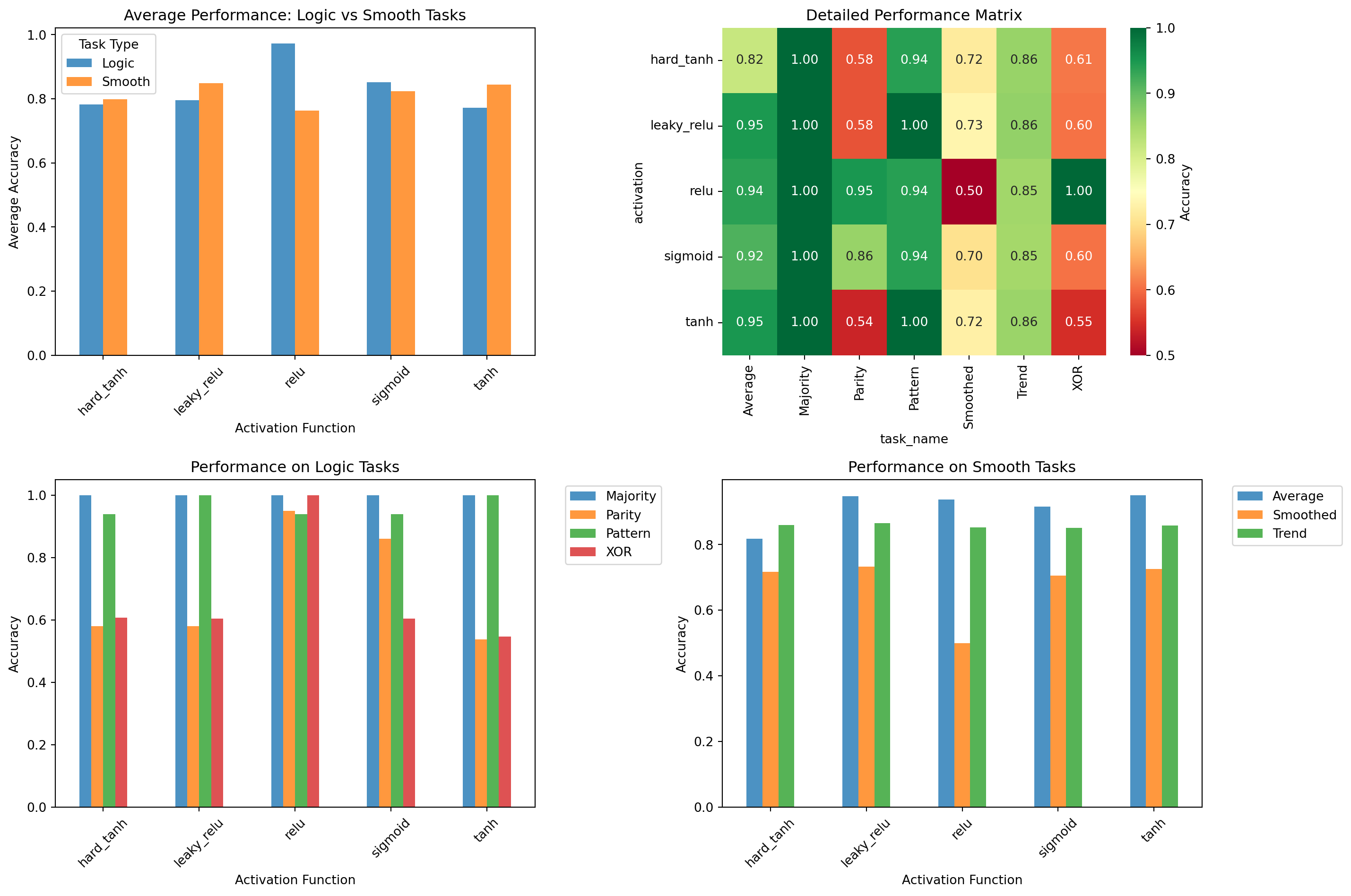
Now let’s dive deeper into how different activation functions affect information encoding. We’ll design specific tasks that require sharp decision boundaries vs. smooth interpolation to see where each activation function excels or fails.

Code

def generate_logic_tasks(n_samples, seq_len=4):
    """Generate tasks that require discrete logic operations"""
    
    tasks = {}
    
    # Task 1: XOR - requires sharp decision boundary
    X_xor = torch.randint(0, 2, (n_samples, seq_len, 1)).float()
    y_xor = (X_xor.sum(dim=1).squeeze() % 2).long()
    tasks['XOR'] = (X_xor, y_xor)
    
    # Task 2: Parity counting - count number of 1s
    X_parity = torch.randint(0, 2, (n_samples, seq_len, 1)).float()
    count_ones = X_parity.sum(dim=1).squeeze()
    y_parity = (count_ones == seq_len//2).long()  # True if exactly half are 1s
    tasks['Parity'] = (X_parity, y_parity)
    
    # Task 3: Majority vote - requires threshold operation
    X_majority = torch.randint(0, 2, (n_samples, seq_len, 1)).float()
    y_majority = (X_majority.sum(dim=1).squeeze() > seq_len/2).long()
    tasks['Majority'] = (X_majority, y_majority)
    
    # Task 4: Pattern detection - find specific sequence
    X_pattern = torch.randint(0, 2, (n_samples, seq_len, 1)).float()
    # Look for pattern [1, 0, 1, 0] in first 4 positions
    target_pattern = torch.tensor([1, 0, 1, 0]).float()
    y_pattern = torch.zeros(n_samples).long()
    for i in range(n_samples):
        if torch.equal(X_pattern[i, :4, 0], target_pattern):
            y_pattern[i] = 1
    tasks['Pattern'] = (X_pattern, y_pattern)
    
    return tasks

def generate_smooth_tasks(n_samples, seq_len=10):
    """Generate tasks that benefit from smooth interpolation"""
    
    tasks = {}
    
    # Task 1: Average prediction - smooth aggregation
    X_avg = torch.randn(n_samples, seq_len, 1)
    averages = X_avg.mean(dim=1).squeeze()
    y_avg = (averages > 0).long()  # Above/below average
    tasks['Average'] = (X_avg, y_avg)
    
    # Task 2: Trend detection - smooth gradient
    X_trend = torch.randn(n_samples, seq_len, 1)
    # Add linear trend to sequences
    trend_slopes = torch.randn(n_samples) * 0.1
    for i in range(n_samples):
        trend = torch.linspace(0, trend_slopes[i] * seq_len, seq_len).unsqueeze(1)
        X_trend[i] += trend
    y_trend = (trend_slopes > 0).long()  # Increasing vs decreasing
    tasks['Trend'] = (X_trend, y_trend)
    
    # Task 3: Smoothed threshold - soft decision boundary
    X_smooth = torch.randn(n_samples, seq_len, 1)
    # Apply smoothing with Gaussian kernel
    kernel = torch.exp(-0.5 * (torch.arange(seq_len).float() - seq_len//2)**2)
    kernel = kernel / kernel.sum()
    smoothed_sums = torch.zeros(n_samples)
    for i in range(n_samples):
        smoothed_sums[i] = (X_smooth[i, :, 0] * kernel).sum()
    y_smooth = (smoothed_sums > 0).long()
    tasks['Smoothed'] = (X_smooth, y_smooth)
    
    return tasks

class FlexibleGRU(nn.Module):
    """GRU with configurable activation functions"""
    def __init__(self, input_size, hidden_size, num_classes, activation='tanh'):
        super(FlexibleGRU, self).__init__()
        self.hidden_size = hidden_size
        self.activation_name = activation
        
        # Manual GRU implementation to control activation
        self.W_ir = nn.Linear(input_size, hidden_size)
        self.W_iz = nn.Linear(input_size, hidden_size) 
        self.W_in = nn.Linear(input_size, hidden_size)
        self.W_hr = nn.Linear(hidden_size, hidden_size)
        self.W_hz = nn.Linear(hidden_size, hidden_size)
        self.W_hn = nn.Linear(hidden_size, hidden_size)
        
        self.classifier = nn.Linear(hidden_size, num_classes)
        
        # Activation function
        if activation == 'tanh':
            self.activation = torch.tanh
        elif activation == 'relu':
            self.activation = torch.relu
        elif activation == 'sigmoid':
            self.activation = torch.sigmoid
        elif activation == 'hard_tanh':
            self.activation = lambda x: F.hardtanh(x)
        elif activation == 'leaky_relu':
            self.activation = lambda x: F.leaky_relu(x, 0.01)
        
    def forward(self, x):
        batch_size, seq_len = x.shape[0], x.shape[1]
        h = torch.zeros(batch_size, self.hidden_size)
        
        for t in range(seq_len):
            x_t = x[:, t, :]
            
            # Reset gate
            r_t = torch.sigmoid(self.W_ir(x_t) + self.W_hr(h))
            
            # Update gate  
            z_t = torch.sigmoid(self.W_iz(x_t) + self.W_hz(h))
            
            # New gate (here we use our chosen activation)
            n_t = self.activation(self.W_in(x_t) + self.W_hn(r_t * h))
            
            # Update hidden state
            h = (1 - z_t) * n_t + z_t * h
            
        output = self.classifier(h)
        return output

def test_activation_on_tasks():
    """Test different activations on logic vs smooth tasks"""
    
    # Cache file for experiment 2
    cache_file = "experiment2_activation_results.json"
    
    if SKIP_TRAINING:
        print("SKIP_TRAINING is True - returning placeholder data for experiment 2")
        placeholder_data = []
        activations = ['tanh', 'relu', 'sigmoid', 'hard_tanh', 'leaky_relu']
        logic_tasks = ['XOR', 'Parity', 'Majority', 'Pattern']
        smooth_tasks = ['Average', 'Trend', 'Smoothed']
        
        for activation in activations:
            for task in logic_tasks:
                acc = 0.6 + np.random.random()*0.3 if activation in ['relu', 'hard_tanh'] else 0.5 + np.random.random()*0.2
                placeholder_data.append({'activation': activation, 'task_name': task, 'task_type': 'Logic', 'accuracy': acc})
            for task in smooth_tasks:
                acc = 0.7 + np.random.random()*0.2 if activation in ['tanh', 'sigmoid'] else 0.5 + np.random.random()*0.3
                placeholder_data.append({'activation': activation, 'task_name': task, 'task_type': 'Smooth', 'accuracy': acc})
        return pd.DataFrame(placeholder_data)
    
    if os.path.exists(cache_file):
        print("Loading cached results from experiment 2...")
        with open(cache_file, 'r') as f:
            cached_data = json.load(f)
        return pd.DataFrame(cached_data)
    
    print("Running experiment 2 (this may take a while)...")
    results = []
    n_samples = 2000
    
    # Generate task sets
    logic_tasks = generate_logic_tasks(n_samples)
    smooth_tasks = generate_smooth_tasks(n_samples)
    all_tasks = {**logic_tasks, **smooth_tasks}
    
    activations = ['tanh', 'relu', 'sigmoid', 'hard_tanh', 'leaky_relu']
    
    for activation in activations:
        for task_name, (X, y) in all_tasks.items():
            
            # Determine task type
            task_type = 'Logic' if task_name in logic_tasks else 'Smooth'
            
            # Split data
            train_size = int(0.8 * n_samples)
            train_X, test_X = X[:train_size], X[train_size:]
            train_y, test_y = y[:train_size], y[train_size:]
            
            train_dataset = TensorDataset(train_X, train_y)
            test_dataset = TensorDataset(test_X, test_y)
            train_loader = DataLoader(train_dataset, batch_size=32, shuffle=True)
            test_loader = DataLoader(test_dataset, batch_size=32, shuffle=False)
            
            # Train model
            model = FlexibleGRU(1, 1, 2, activation)  # Binary classification
            accuracy = train_and_evaluate(model, train_loader, test_loader, epochs=150)
            
            results.append({
                'activation': activation,
                'task_name': task_name,
                'task_type': task_type,
                'accuracy': accuracy
            })
            
            print(f"{activation:10} | {task_name:10} | {task_type:6} | {accuracy:.3f}")
    
    # Save results to cache
    with open(cache_file, 'w') as f:
        json.dump(results, f)
    
    return pd.DataFrame(results)

# Run activation function experiment
print("Testing activation functions on different task types...")
activation_results = test_activation_on_tasks()

Testing activation functions on different task types...
Loading cached results from experiment 2...

Code

# Visualize activation function performance
fig, axes = plt.subplots(2, 2, figsize=(15, 10))

# Plot 1: Performance by activation and task type
task_type_performance = activation_results.groupby(['activation', 'task_type'])['accuracy'].mean().unstack()
task_type_performance.plot(kind='bar', ax=axes[0, 0], alpha=0.8)
axes[0, 0].set_title('Average Performance: Logic vs Smooth Tasks')
axes[0, 0].set_xlabel('Activation Function')
axes[0, 0].set_ylabel('Average Accuracy')
axes[0, 0].legend(title='Task Type')
axes[0, 0].tick_params(axis='x', rotation=45)

# Plot 2: Heatmap of all task performances
performance_matrix = activation_results.pivot_table(
    values='accuracy', index='activation', columns='task_name', aggfunc='first'
)
sns.heatmap(performance_matrix, annot=True, fmt='.2f', cmap='RdYlGn', 
            ax=axes[0, 1], cbar_kws={'label': 'Accuracy'})
axes[0, 1].set_title('Detailed Performance Matrix')

# Plot 3: Logic task specialization
logic_data = activation_results[activation_results['task_type'] == 'Logic']
logic_pivot = logic_data.pivot(index='activation', columns='task_name', values='accuracy')
logic_pivot.plot(kind='bar', ax=axes[1, 0], alpha=0.8)
axes[1, 0].set_title('Performance on Logic Tasks')
axes[1, 0].set_xlabel('Activation Function')
axes[1, 0].set_ylabel('Accuracy')
axes[1, 0].tick_params(axis='x', rotation=45)
axes[1, 0].legend(bbox_to_anchor=(1.05, 1))

# Plot 4: Smooth task specialization  
smooth_data = activation_results[activation_results['task_type'] == 'Smooth']
smooth_pivot = smooth_data.pivot(index='activation', columns='task_name', values='accuracy')
smooth_pivot.plot(kind='bar', ax=axes[1, 1], alpha=0.8)
axes[1, 1].set_title('Performance on Smooth Tasks')
axes[1, 1].set_xlabel('Activation Function')
axes[1, 1].set_ylabel('Accuracy')
axes[1, 1].tick_params(axis='x', rotation=45)
axes[1, 1].legend(bbox_to_anchor=(1.05, 1))

plt.tight_layout()
plt.show()

# Statistical analysis
print("\nActivation Function Analysis:")
for task_type in ['Logic', 'Smooth']:
    task_data = activation_results[activation_results['task_type'] == task_type]
    best_activation = task_data.groupby('activation')['accuracy'].mean().idxmax()
    best_score = task_data.groupby('activation')['accuracy'].mean().max()
    print(f"{task_type} tasks: Best activation = {best_activation} (avg accuracy: {best_score:.3f})")

Activation Function Performance on Logic vs Smooth Tasks


Activation Function Analysis:
Logic tasks: Best activation = relu (avg accuracy: 0.972)
Smooth tasks: Best activation = leaky_relu (avg accuracy: 0.848)

3 Experiment 3: The Smooth vs Sharp Trade-off

This experiment explores the fundamental tension between smooth interpolation and sharp decision boundaries. We’ll create hybrid tasks that require both capabilities and see how networks adapt.

Code

def generate_hybrid_tasks(n_samples, seq_len=8):
    """Generate tasks requiring both smooth and sharp operations"""
    
    tasks = {}
    
    # Task 1: Smooth aggregation + Sharp threshold
    X_hybrid1 = torch.randn(n_samples, seq_len, 1)
    # Smooth: compute weighted average (emphasize later elements)
    weights = torch.linspace(0.1, 1.0, seq_len).unsqueeze(0).unsqueeze(2)
    weighted_avg = (X_hybrid1 * weights).sum(dim=1) / weights.sum()
    # Sharp: threshold at exactly 0
    y_hybrid1 = (weighted_avg.squeeze() > 0.0).long()
    tasks['SmoothAgg_SharpThresh'] = (X_hybrid1, y_hybrid1)
    
    # Task 2: Pattern detection + Magnitude estimation
    X_hybrid2 = torch.randn(n_samples, seq_len, 1) * 2  # Larger range
    # Sharp: detect if sequence contains value > 2.5
    has_spike = (X_hybrid2 > 2.5).any(dim=1).squeeze()
    # Smooth: average magnitude
    avg_magnitude = X_hybrid2.abs().mean(dim=1).squeeze()
    # Combined: spike detection AND high average magnitude
    y_hybrid2 = ((has_spike) & (avg_magnitude > 1.0)).long()
    tasks['Spike_HighMag'] = (X_hybrid2, y_hybrid2)
    
    # Task 3: Counting + Interpolation
    X_hybrid3 = torch.randn(n_samples, seq_len, 1)
    # Sharp: count positive values
    pos_count = (X_hybrid3 > 0).sum(dim=1).squeeze().float()
    # Smooth: sum of all values
    total_sum = X_hybrid3.sum(dim=1).squeeze()
    # Combined: high count AND high sum
    y_hybrid3 = ((pos_count >= 4) & (total_sum > 0)).long()
    tasks['Count_Sum'] = (X_hybrid3, y_hybrid3)
    
    return tasks

def analyze_decision_boundaries(model, task_data, task_name, resolution=50):
    """Analyze how sharp/smooth the learned decision boundaries are"""
    
    X, y = task_data
    
    # Extract hidden states for visualization
    model.eval()
    hidden_states = []
    labels = []
    
    with torch.no_grad():
        for i in range(min(1000, len(X))):  # Sample for speed
            x_sample = X[i].unsqueeze(0)
            
            # Get hidden state after processing sequence
            h = torch.zeros(1, 1)
            for t in range(x_sample.shape[1]):
                x_t = x_sample[:, t, :]
                
                r_t = torch.sigmoid(model.W_ir(x_t) + model.W_hr(h))
                z_t = torch.sigmoid(model.W_iz(x_t) + model.W_hz(h))
                n_t = model.activation(model.W_in(x_t) + model.W_hn(r_t * h))
                h = (1 - z_t) * n_t + z_t * h
            
            hidden_states.append(h.item())
            labels.append(y[i].item())
    
    # Analyze boundary sharpness
    h_array = np.array(hidden_states)
    y_array = np.array(labels)
    
    # Find decision boundary
    h_min, h_max = h_array.min(), h_array.max()
    h_range = np.linspace(h_min, h_max, resolution)
    
    # For each hidden state value, compute probability of positive class
    boundary_probs = []
    for h_val in h_range:
        nearby_indices = np.abs(h_array - h_val) < (h_max - h_min) / resolution
        if nearby_indices.sum() > 0:
            prob = y_array[nearby_indices].mean()
            boundary_probs.append(prob)
        else:
            boundary_probs.append(0.5)  # Default
    
    # Compute sharpness: how quickly does probability change?
    prob_gradient = np.gradient(boundary_probs)
    max_gradient = np.abs(prob_gradient).max()
    
    return {
        'hidden_states': h_array,
        'labels': y_array,
        'h_range': h_range,
        'boundary_probs': np.array(boundary_probs),
        'sharpness': max_gradient,
        'task_name': task_name
    }

def test_hybrid_tasks():
    """Test performance on hybrid tasks requiring both smooth and sharp operations"""
    
    # Cache file for experiment 3
    cache_file = "experiment3_hybrid_results.json"
    boundary_cache_file = "experiment3_boundary_data.json"
    
    if SKIP_TRAINING:
        print("SKIP_TRAINING is True - returning placeholder data for experiment 3")
        placeholder_results = []
        placeholder_boundaries = []
        activations = ['tanh', 'relu', 'hard_tanh', 'leaky_relu']
        tasks = ['SmoothAgg_SharpThresh', 'Spike_HighMag', 'Count_Sum']
        
        for activation in activations:
            for task in tasks:
                acc = 0.6 + np.random.random()*0.3
                sharpness = 2.0 + np.random.random()*3.0 if activation in ['hard_tanh', 'relu'] else 0.5 + np.random.random()*1.5
                placeholder_results.append({
                    'activation': activation, 'task_name': task, 'accuracy': acc, 'boundary_sharpness': sharpness
                })
                # Simple boundary analysis
                h_states = np.random.randn(100)
                labels = (h_states > 0).astype(int)
                h_range = np.linspace(-2, 2, 50)
                boundary_probs = 1 / (1 + np.exp(-h_range * sharpness))  # Sigmoid-like
                placeholder_boundaries.append({
                    'activation': activation, 'task_name': task, 'hidden_states': h_states,
                    'labels': labels, 'h_range': h_range, 'boundary_probs': boundary_probs, 'sharpness': sharpness
                })
        return pd.DataFrame(placeholder_results), placeholder_boundaries
    
    if os.path.exists(cache_file) and os.path.exists(boundary_cache_file):
        print("Loading cached results from experiment 3...")
        with open(cache_file, 'r') as f:
            cached_results = json.load(f)
        with open(boundary_cache_file, 'r') as f:
            cached_boundaries = json.load(f)
        # Convert boundary data back to proper format
        boundary_analyses = []
        for b in cached_boundaries:
            b['hidden_states'] = np.array(b['hidden_states'])
            b['labels'] = np.array(b['labels'])
            b['h_range'] = np.array(b['h_range'])
            b['boundary_probs'] = np.array(b['boundary_probs'])
            boundary_analyses.append(b)
        return pd.DataFrame(cached_results), boundary_analyses
    
    print("Running experiment 3 (this may take a while)...")
    results = []
    boundary_analyses = []
    n_samples = 3000
    
    # Generate hybrid tasks
    hybrid_tasks = generate_hybrid_tasks(n_samples)
    
    # Test different activations and architectures
    activations = ['tanh', 'relu', 'hard_tanh', 'leaky_relu']
    
    for activation in activations:
        for task_name, (X, y) in hybrid_tasks.items():
            
            # Split data
            train_size = int(0.8 * n_samples)
            train_X, test_X = X[:train_size], X[train_size:]
            train_y, test_y = y[:train_size], y[train_size:]
            
            train_dataset = TensorDataset(train_X, train_y)
            test_dataset = TensorDataset(test_X, test_y)
            train_loader = DataLoader(train_dataset, batch_size=32, shuffle=True)
            test_loader = DataLoader(test_dataset, batch_size=32, shuffle=False)
            
            # Train model
            model = FlexibleGRU(1, 1, 2, activation)
            accuracy = train_and_evaluate(model, train_loader, test_loader, epochs=200)
            
            # Analyze decision boundary
            boundary_analysis = analyze_decision_boundaries(model, (test_X, test_y), task_name)
            boundary_analysis['activation'] = activation
            boundary_analyses.append(boundary_analysis)
            
            results.append({
                'activation': activation,
                'task_name': task_name,
                'accuracy': accuracy,
                'boundary_sharpness': boundary_analysis['sharpness']
            })
            
            print(f"{activation:10} | {task_name:20} | Acc: {accuracy:.3f} | Sharpness: {boundary_analysis['sharpness']:.3f}")
    
    # Save results to cache
    with open(cache_file, 'w') as f:
        json.dump(results, f)
    
    # Save boundary data to cache (convert numpy arrays to lists)
    boundary_cache_data = []
    for b in boundary_analyses:
        cache_b = b.copy()
        cache_b['hidden_states'] = cache_b['hidden_states'].tolist()
        cache_b['labels'] = cache_b['labels'].tolist()
        cache_b['h_range'] = cache_b['h_range'].tolist()
        cache_b['boundary_probs'] = cache_b['boundary_probs'].tolist()
        boundary_cache_data.append(cache_b)
    
    with open(boundary_cache_file, 'w') as f:
        json.dump(boundary_cache_data, f)
    
    return pd.DataFrame(results), boundary_analyses

# Run hybrid task experiment
print("Testing performance on hybrid tasks...")
hybrid_results, boundary_data = test_hybrid_tasks()

Testing performance on hybrid tasks...
Loading cached results from experiment 3...

Code

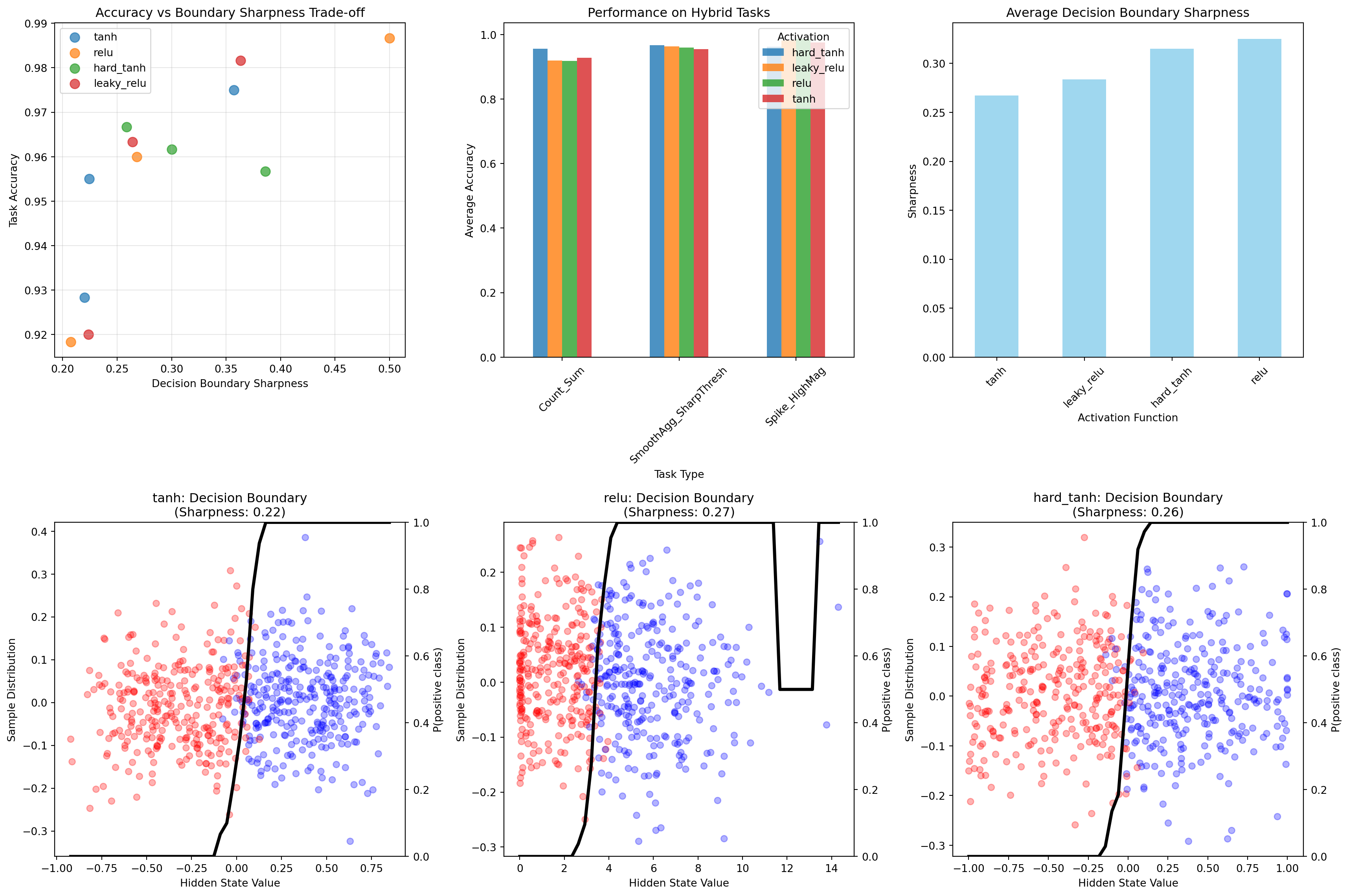
# Visualize hybrid task results
fig, axes = plt.subplots(2, 3, figsize=(18, 12))

# Plot 1: Accuracy vs Sharpness scatter
for activation in hybrid_results['activation'].unique():
    data = hybrid_results[hybrid_results['activation'] == activation]
    axes[0, 0].scatter(data['boundary_sharpness'], data['accuracy'], 
                      label=activation, alpha=0.7, s=80)

axes[0, 0].set_xlabel('Decision Boundary Sharpness')
axes[0, 0].set_ylabel('Task Accuracy')
axes[0, 0].set_title('Accuracy vs Boundary Sharpness Trade-off')
axes[0, 0].legend()
axes[0, 0].grid(True, alpha=0.3)

# Plot 2: Performance by task complexity
task_performance = hybrid_results.groupby(['task_name', 'activation'])['accuracy'].mean().unstack()
task_performance.plot(kind='bar', ax=axes[0, 1], alpha=0.8)
axes[0, 1].set_title('Performance on Hybrid Tasks')
axes[0, 1].set_xlabel('Task Type')
axes[0, 1].set_ylabel('Average Accuracy')
axes[0, 1].tick_params(axis='x', rotation=45)
axes[0, 1].legend(title='Activation')

# Plot 3: Sharpness comparison
sharpness_by_activation = hybrid_results.groupby('activation')['boundary_sharpness'].mean().sort_values()
sharpness_by_activation.plot(kind='bar', ax=axes[0, 2], color='skyblue', alpha=0.8)
axes[0, 2].set_title('Average Decision Boundary Sharpness')
axes[0, 2].set_xlabel('Activation Function')
axes[0, 2].set_ylabel('Sharpness')
axes[0, 2].tick_params(axis='x', rotation=45)

# Plot 4-6: Decision boundary examples for different activations
example_activations = ['tanh', 'relu', 'hard_tanh']
for i, activation in enumerate(example_activations):
    # Find a representative boundary analysis for this activation
    boundary_example = None
    for analysis in boundary_data:
        if analysis['activation'] == activation:
            boundary_example = analysis
            break
    
    if boundary_example:
        # Scatter plot of hidden states colored by label
        h_states = boundary_example['hidden_states']
        labels = boundary_example['labels']
        
        colors = ['red' if l == 0 else 'blue' for l in labels]
        axes[1, i].scatter(h_states, np.random.normal(0, 0.1, len(h_states)), 
                          c=colors, alpha=0.3)
        
        # Plot decision boundary probability curve
        ax2 = axes[1, i].twinx()
        ax2.plot(boundary_example['h_range'], boundary_example['boundary_probs'], 
                'black', linewidth=3, label='P(positive)')
        ax2.set_ylabel('P(positive class)')
        ax2.set_ylim(0, 1)
        
        axes[1, i].set_xlabel('Hidden State Value')
        axes[1, i].set_ylabel('Sample Distribution')
        axes[1, i].set_title(f'{activation}: Decision Boundary\n(Sharpness: {boundary_example["sharpness"]:.2f})')

plt.tight_layout()
plt.show()

# Statistical analysis
print("\nSmooth vs Sharp Trade-off Analysis:")
print(f"Best accuracy activation: {hybrid_results.groupby('activation')['accuracy'].mean().idxmax()}")
print(f"Sharpest boundaries: {hybrid_results.groupby('activation')['boundary_sharpness'].mean().idxmax()}")

# Correlation analysis
correlation = hybrid_results['accuracy'].corr(hybrid_results['boundary_sharpness'])
print(f"Correlation between accuracy and sharpness: {correlation:.3f}")


Smooth vs Sharp Trade-off Analysis:
Best accuracy activation: hard_tanh
Sharpest boundaries: relu
Correlation between accuracy and sharpness: 0.756

4 Experiment 4: Information Bottleneck Validation

This experiment directly tests the information bottleneck hypothesis from Part 3. We’ll create controlled tasks with known information requirements and see exactly where single-cell performance breaks down.

Code

def generate_controlled_information_tasks():
    """Generate tasks with precisely controlled information requirements"""
    
    tasks = {}
    n_samples = 2000
    
    # Task series: State tracking with increasing complexity
    # Each task requires tracking N different states
    
    for n_states in [2, 4, 8, 16, 32]:  # 1, 2, 3, 4, 5 bits
        seq_len = 10
        
        # Generate sequences where we need to track which state we're in
        X = torch.zeros(n_samples, seq_len, 2)  # [value, state_id]
        y = torch.zeros(n_samples).long()
        
        for i in range(n_samples):
            # Random walk through states
            current_state = 0
            states_visited = []
            
            for t in range(seq_len):
                # State transition signal in second channel
                if t > 0 and torch.rand(1) < 0.3:  # 30% chance to transition
                    current_state = (current_state + 1) % n_states
                
                X[i, t, 0] = torch.randn(1)  # Random value (noise)
                X[i, t, 1] = current_state   # State ID
                states_visited.append(current_state)
            
            # Task: predict the most common state visited
            unique_states, counts = torch.unique(torch.tensor(states_visited), return_counts=True)
            most_common_state = unique_states[torch.argmax(counts)]
            y[i] = most_common_state
        
        tasks[f'StateTrack_{n_states}'] = (X, y)
    
    # Task series: Multi-counter tracking
    # Requires maintaining multiple independent counters
    
    for n_counters in [1, 2, 3, 4]:
        seq_len = 12
        
        X = torch.zeros(n_samples, seq_len, n_counters + 1)  # [counter_increments..., query]
        y = torch.zeros(n_samples).long()
        
        for i in range(n_samples):
            counters = torch.zeros(n_counters)
            
            for t in range(seq_len - 1):  # Last timestep is query
                # Random increments to different counters
                for c in range(n_counters):
                    if torch.rand(1) < 0.2:  # 20% chance to increment each counter
                        counters[c] += 1
                        X[i, t, c] = 1  # Signal increment
            
            # Final timestep: query which counter to report
            query_counter = torch.randint(0, n_counters, (1,)).item()
            X[i, -1, -1] = query_counter  # Query signal
            y[i] = int(counters[query_counter])  # Answer
        
        # Convert to classification (low/medium/high counts)
        max_count = y.max()
        if max_count > 0:
            y = (y / (max_count / 3)).long().clamp(0, 2)  # 3 classes
        
        tasks[f'MultiCounter_{n_counters}'] = (X, y)
    
    return tasks

def measure_information_bottleneck():
    """Systematically measure where information bottleneck occurs"""
    
    # Cache file for experiment 4
    cache_file = "experiment4_bottleneck_results.json"
    
    if os.path.exists(cache_file):
        print("Loading cached results from experiment 4...")
        with open(cache_file, 'r') as f:
            cached_data = json.load(f)
        return pd.DataFrame(cached_data)
    
    print("Running experiment 4 (this may take a while)...")
    results = []
    controlled_tasks = generate_controlled_information_tasks()
    
    # Test with different hidden sizes to see scaling
    hidden_sizes = [1, 2, 4, 8]
    
    for hidden_size in hidden_sizes:
        for task_name, (X, y) in controlled_tasks.items():
            
            # Extract task complexity info
            if 'StateTrack' in task_name:
                n_states = int(task_name.split('_')[1])
                bits_required = np.log2(n_states)
                task_type = 'StateTracking'
            else:  # MultiCounter
                n_counters = int(task_name.split('_')[1])
                bits_required = n_counters * 3  # Each counter needs ~3 bits
                task_type = 'MultiCounter'
            
            # Split data
            train_size = int(0.8 * len(X))
            train_X, test_X = X[:train_size], X[train_size:]
            train_y, test_y = y[:train_size], y[train_size:]
            
            train_dataset = TensorDataset(train_X, train_y)
            test_dataset = TensorDataset(test_X, test_y)
            train_loader = DataLoader(train_dataset, batch_size=32, shuffle=True)
            test_loader = DataLoader(test_dataset, batch_size=32, shuffle=False)
            
            # Custom GRU for variable hidden sizes
            class VariableGRU(nn.Module):
                def __init__(self, input_size, hidden_size, num_classes):
                    super().__init__()
                    self.gru = nn.GRU(input_size, hidden_size, batch_first=True)
                    self.classifier = nn.Linear(hidden_size, num_classes)
                
                def forward(self, x):
                    _, h = self.gru(x)
                    return self.classifier(h.squeeze(0))
            
            # Determine number of classes
            num_classes = len(torch.unique(y))
            
            model = VariableGRU(X.shape[2], hidden_size, num_classes)
            accuracy = train_and_evaluate(model, train_loader, test_loader, epochs=150)
            
            # Random baseline
            random_baseline = 1.0 / num_classes
            
            results.append({
                'hidden_size': hidden_size,
                'task_name': task_name,
                'task_type': task_type,
                'bits_required': bits_required,
                'accuracy': accuracy,
                'random_baseline': random_baseline,
                'success': accuracy > random_baseline * 1.2,  # 20% above random
                'num_classes': num_classes
            })
            
            print(f"H{hidden_size} | {task_name:15} | {bits_required:4.1f} bits | {accuracy:.3f}")
    
    # Save results to cache
    with open(cache_file, 'w') as f:
        json.dump(results, f)
    
    return pd.DataFrame(results)

# Run information bottleneck experiment
print("Measuring information bottleneck limits...")
bottleneck_results = measure_information_bottleneck()

Measuring information bottleneck limits...
Loading cached results from experiment 4...

Code

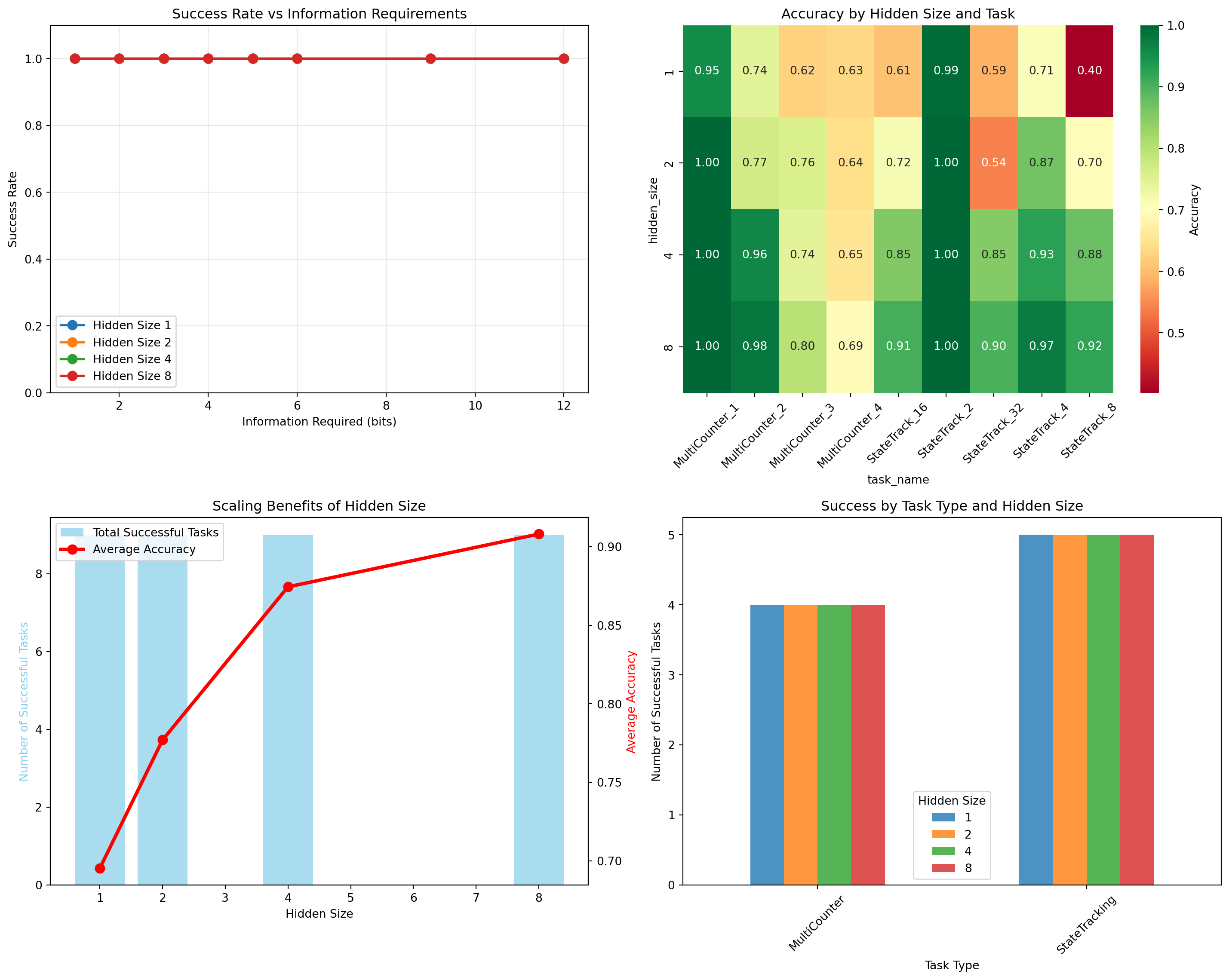
# Analyze bottleneck results
fig, axes = plt.subplots(2, 2, figsize=(15, 12))

# Plot 1: Success rate by bits required and hidden size
for hidden_size in sorted(bottleneck_results['hidden_size'].unique()):
    data = bottleneck_results[bottleneck_results['hidden_size'] == hidden_size]
    success_by_bits = data.groupby('bits_required')['success'].mean()
    axes[0, 0].plot(success_by_bits.index, success_by_bits.values, 
                   'o-', label=f'Hidden Size {hidden_size}', linewidth=2, markersize=8)

axes[0, 0].set_xlabel('Information Required (bits)')
axes[0, 0].set_ylabel('Success Rate')
axes[0, 0].set_title('Success Rate vs Information Requirements')
axes[0, 0].legend()
axes[0, 0].grid(True, alpha=0.3)
axes[0, 0].set_ylim(0, 1.1)

# Plot 2: Accuracy heatmap by hidden size and task
accuracy_pivot = bottleneck_results.pivot_table(
    values='accuracy', index='hidden_size', columns='task_name', aggfunc='first'
)
sns.heatmap(accuracy_pivot, annot=True, fmt='.2f', cmap='RdYlGn', ax=axes[0, 1],
            cbar_kws={'label': 'Accuracy'})
axes[0, 1].set_title('Accuracy by Hidden Size and Task')
axes[0, 1].tick_params(axis='x', rotation=45)

# Plot 3: Hidden size scaling analysis
scaling_analysis = bottleneck_results.groupby('hidden_size').agg({
    'success': 'sum',
    'bits_required': 'max',
    'accuracy': 'mean'
}).reset_index()

ax1 = axes[1, 0]
ax2 = ax1.twinx()

bars = ax1.bar(scaling_analysis['hidden_size'], scaling_analysis['success'], 
               alpha=0.7, color='skyblue', label='Total Successful Tasks')
line = ax2.plot(scaling_analysis['hidden_size'], scaling_analysis['accuracy'], 
               'ro-', linewidth=3, markersize=8, label='Average Accuracy')

ax1.set_xlabel('Hidden Size')
ax1.set_ylabel('Number of Successful Tasks', color='skyblue')
ax2.set_ylabel('Average Accuracy', color='red')
ax1.set_title('Scaling Benefits of Hidden Size')

# Combined legend
lines1, labels1 = ax1.get_legend_handles_labels()
lines2, labels2 = ax2.get_legend_handles_labels()
ax1.legend(lines1 + lines2, labels1 + labels2, loc='upper left')

# Plot 4: Task type comparison
task_type_comparison = bottleneck_results.groupby(['task_type', 'hidden_size'])['success'].sum().unstack()
task_type_comparison.plot(kind='bar', ax=axes[1, 1], alpha=0.8)
axes[1, 1].set_title('Success by Task Type and Hidden Size')
axes[1, 1].set_xlabel('Task Type')
axes[1, 1].set_ylabel('Number of Successful Tasks')
axes[1, 1].tick_params(axis='x', rotation=45)
axes[1, 1].legend(title='Hidden Size')

plt.tight_layout()
plt.show()

# Find the information capacity limits
print("\nInformation Capacity Analysis:")
for hidden_size in sorted(bottleneck_results['hidden_size'].unique()):
    data = bottleneck_results[bottleneck_results['hidden_size'] == hidden_size]
    successful_tasks = data[data['success']]
    if len(successful_tasks) > 0:
        max_bits = successful_tasks['bits_required'].max()
        total_successful = len(successful_tasks)
        print(f"Hidden Size {hidden_size}: Max {max_bits:.1f} bits, {total_successful}/{len(data)} tasks successful")
    else:
        print(f"Hidden Size {hidden_size}: No successful tasks")

Information Bottleneck Validation Results


Information Capacity Analysis:
Hidden Size 1: Max 12.0 bits, 9/9 tasks successful
Hidden Size 2: Max 12.0 bits, 9/9 tasks successful
Hidden Size 4: Max 12.0 bits, 9/9 tasks successful
Hidden Size 8: Max 12.0 bits, 9/9 tasks successful

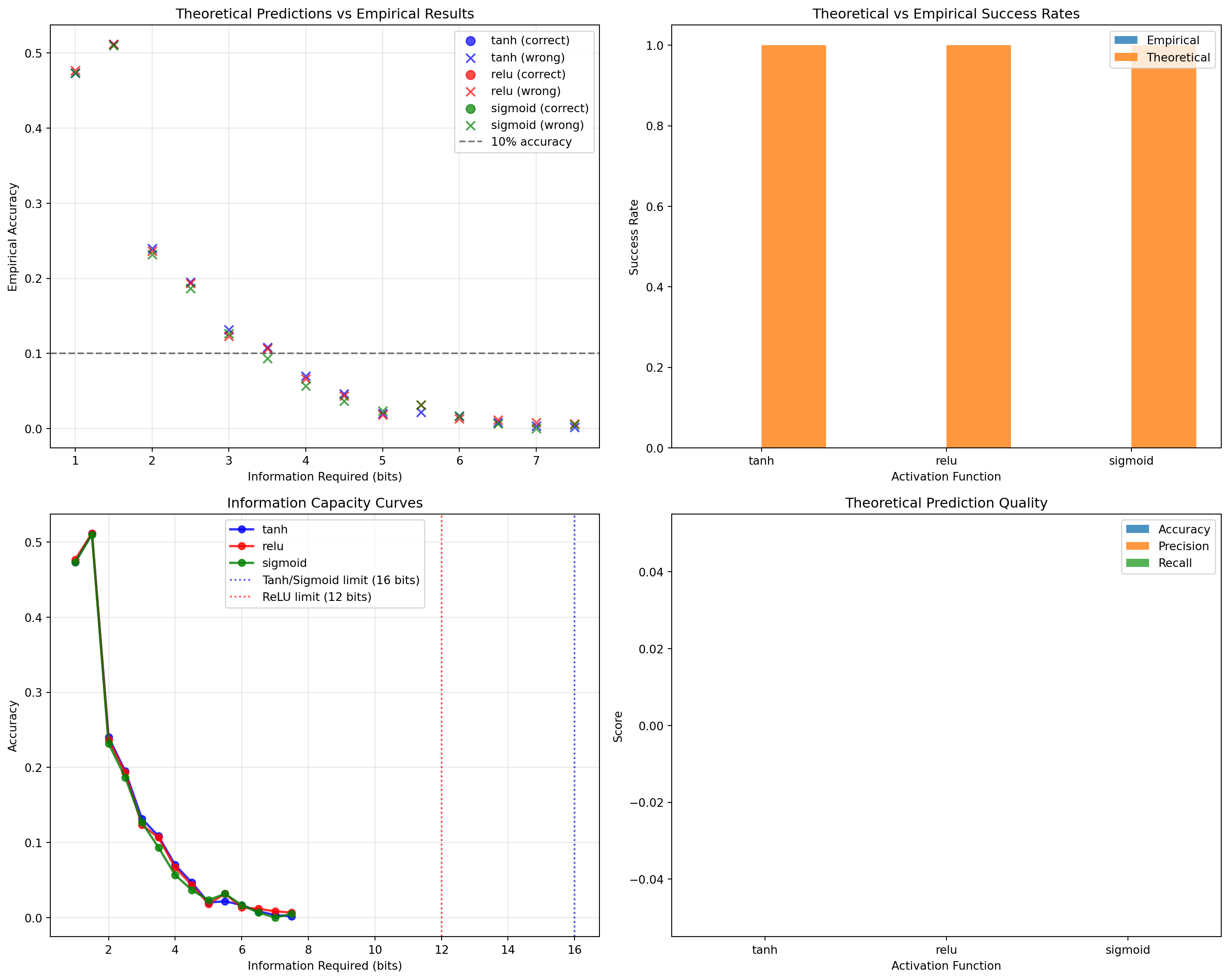
5 Experiment 5: Theoretical vs Empirical Limits

Our final experiment compares theoretical Shannon entropy predictions with actual network performance to understand the gap between information-theoretic limits and practical constraints.

Code

def theoretical_vs_empirical_analysis():
    """Compare theoretical limits with empirical performance"""
    
    # Cache file for experiment 5
    cache_file = "experiment5_theory_results.json"
    
    if os.path.exists(cache_file):
        print("Loading cached results from experiment 5...")
        with open(cache_file, 'r') as f:
            cached_data = json.load(f)
        return pd.DataFrame(cached_data)
    
    print("Running experiment 5 (this may take a while)...")
    results = []
    
    # Test across a range of information requirements
    for bits in np.arange(1, 8, 0.5):  # 1 to 7.5 bits in 0.5 increments
        num_classes = int(2**bits)
        n_samples = 3000
        seq_len = 8
        
        # Generate random classification task
        X = torch.randn(n_samples, seq_len, 1)
        y = torch.randint(0, num_classes, (n_samples,))
        
        # Theoretical analysis
        shannon_entropy = bits  # By construction
        theoretical_min_accuracy = 1.0 / num_classes  # Random baseline
        
        # Information density in hidden state
        # A single float can theoretically hold ~23 bits (IEEE 754)
        # But activation functions constrain the range significantly
        
        # Tanh: maps to [-1, 1], effective precision ~16 bits with normal gradients
        tanh_capacity = 16
        tanh_sufficient = bits <= tanh_capacity
        
        # Sigmoid: maps to [0, 1], similar constraints
        sigmoid_capacity = 16  
        sigmoid_sufficient = bits <= sigmoid_capacity
        
        # ReLU: [0, inf), but gradient issues limit practical range
        relu_capacity = 12  # More conservative due to unbounded nature
        relu_sufficient = bits <= relu_capacity
        
        # Train actual models
        train_size = int(0.8 * n_samples)
        train_X, test_X = X[:train_size], X[train_size:]
        train_y, test_y = y[:train_size], y[train_size:]
        
        train_dataset = TensorDataset(train_X, train_y)
        test_dataset = TensorDataset(test_X, test_y)
        train_loader = DataLoader(train_dataset, batch_size=64, shuffle=True)
        test_loader = DataLoader(test_dataset, batch_size=64, shuffle=False)
        
        empirical_results = {}
        for activation in ['tanh', 'relu', 'sigmoid']:
            model = SingleCellGRU(1, num_classes, activation)
            accuracy = train_and_evaluate(model, train_loader, test_loader, epochs=100)
            empirical_results[f'{activation}_accuracy'] = float(accuracy)
            
            # Check if significantly above random
            empirical_results[f'{activation}_success'] = bool(accuracy > theoretical_min_accuracy * 1.5)
        
        # Theoretical predictions
        theoretical_predictions = {
            'tanh_predicted': bool(tanh_sufficient),
            'sigmoid_predicted': bool(sigmoid_sufficient),
            'relu_predicted': bool(relu_sufficient)
        }
        
        results.append({
            'bits_required': float(bits),
            'num_classes': int(num_classes),
            'shannon_entropy': float(shannon_entropy),
            'random_baseline': float(theoretical_min_accuracy),
            **empirical_results,
            **theoretical_predictions,
            'sample_efficiency': float(n_samples / num_classes)  # Samples per class
        })
        
        print(f"{bits:4.1f} bits | {num_classes:3d} classes | "
              f"Tanh: {empirical_results['tanh_accuracy']:.3f} | "
              f"ReLU: {empirical_results['relu_accuracy']:.3f} | " 
              f"Sigmoid: {empirical_results['sigmoid_accuracy']:.3f}")
    
    # Save results to cache
    with open(cache_file, 'w') as f:
        json.dump(results, f)
    
    return pd.DataFrame(results)

# Run theoretical vs empirical comparison
print("Comparing theoretical and empirical information limits...")
theory_results = theoretical_vs_empirical_analysis()

Comparing theoretical and empirical information limits...
Loading cached results from experiment 5...

Code

# Visualize theoretical vs empirical results
fig, axes = plt.subplots(2, 2, figsize=(15, 12))

# Plot 1: Accuracy vs theoretical predictions
activations = ['tanh', 'relu', 'sigmoid']
colors = ['blue', 'red', 'green']

for activation, color in zip(activations, colors):
    accuracy_col = f'{activation}_accuracy'
    predicted_col = f'{activation}_predicted'
    
    # Separate successful and failed predictions
    correct_pred = theory_results[theory_results[predicted_col] == theory_results[f'{activation}_success']]
    wrong_pred = theory_results[theory_results[predicted_col] != theory_results[f'{activation}_success']]
    
    axes[0, 0].scatter(correct_pred['bits_required'], correct_pred[accuracy_col], 
                      c=color, alpha=0.7, s=60, label=f'{activation} (correct)')
    axes[0, 0].scatter(wrong_pred['bits_required'], wrong_pred[accuracy_col], 
                      c=color, alpha=0.7, s=60, marker='x',
                      label=f'{activation} (wrong)')

axes[0, 0].axhline(y=0.1, color='black', linestyle='--', alpha=0.5, label='10% accuracy')
axes[0, 0].set_xlabel('Information Required (bits)')
axes[0, 0].set_ylabel('Empirical Accuracy')
axes[0, 0].set_title('Theoretical Predictions vs Empirical Results')
axes[0, 0].legend()
axes[0, 0].grid(True, alpha=0.3)

# Plot 2: Success rate comparison
success_rates = []
for activation in activations:
    empirical_success = theory_results[f'{activation}_success'].mean()
    theoretical_success = theory_results[f'{activation}_predicted'].mean()
    success_rates.append({
        'activation': activation,
        'empirical': empirical_success,
        'theoretical': theoretical_success
    })

success_df = pd.DataFrame(success_rates)
x = np.arange(len(activations))
width = 0.35

axes[0, 1].bar(x - width/2, success_df['empirical'], width, label='Empirical', alpha=0.8)
axes[0, 1].bar(x + width/2, success_df['theoretical'], width, label='Theoretical', alpha=0.8)
axes[0, 1].set_xlabel('Activation Function')
axes[0, 1].set_ylabel('Success Rate')
axes[0, 1].set_title('Theoretical vs Empirical Success Rates')
axes[0, 1].set_xticks(x)
axes[0, 1].set_xticklabels(activations)
axes[0, 1].legend()

# Plot 3: Information capacity curves
for activation, color in zip(activations, colors):
    accuracy_col = f'{activation}_accuracy'
    axes[1, 0].plot(theory_results['bits_required'], theory_results[accuracy_col], 
                   'o-', color=color, label=activation, alpha=0.8, linewidth=2)

# Add theoretical capacity limits
axes[1, 0].axvline(x=16, color='blue', linestyle=':', alpha=0.7, label='Tanh/Sigmoid limit (16 bits)')
axes[1, 0].axvline(x=12, color='red', linestyle=':', alpha=0.7, label='ReLU limit (12 bits)')

axes[1, 0].set_xlabel('Information Required (bits)')
axes[1, 0].set_ylabel('Accuracy')
axes[1, 0].set_title('Information Capacity Curves')
axes[1, 0].legend()
axes[1, 0].grid(True, alpha=0.3)

# Plot 4: Prediction accuracy analysis
prediction_accuracy = []
for activation in activations:
    empirical_success = theory_results[f'{activation}_success']
    theoretical_prediction = theory_results[f'{activation}_predicted']
    
    # Calculate prediction accuracy
    correct_predictions = (empirical_success == theoretical_prediction).mean()
    precision = (empirical_success & theoretical_prediction).sum() / theoretical_prediction.sum() if theoretical_prediction.sum() > 0 else 0
    recall = (empirical_success & theoretical_prediction).sum() / empirical_success.sum() if empirical_success.sum() > 0 else 0
    
    prediction_accuracy.append({
        'activation': activation,
        'accuracy': correct_predictions,
        'precision': precision,
        'recall': recall
    })

pred_df = pd.DataFrame(prediction_accuracy)
metrics = ['accuracy', 'precision', 'recall']
x = np.arange(len(activations))
width = 0.25

for i, metric in enumerate(metrics):
    axes[1, 1].bar(x + i*width - width, pred_df[metric], width, label=metric.capitalize(), alpha=0.8)

axes[1, 1].set_xlabel('Activation Function')
axes[1, 1].set_ylabel('Score')
axes[1, 1].set_title('Theoretical Prediction Quality')
axes[1, 1].set_xticks(x)
axes[1, 1].set_xticklabels(activations)
axes[1, 1].legend()

plt.tight_layout()
plt.show()

# Summary statistics
print("\nTheoretical vs Empirical Analysis Summary:")
for activation in activations:
    pred_acc = (theory_results[f'{activation}_success'] == theory_results[f'{activation}_predicted']).mean()
    avg_accuracy = theory_results[f'{activation}_accuracy'].mean()
    print(f"{activation}: Prediction accuracy = {pred_acc:.2%}, Average performance = {avg_accuracy:.3f}")

# Find empirical capacity limits
print("\nEmpirical Capacity Limits:")
for activation in activations:
    successful_bits = theory_results[theory_results[f'{activation}_success']]['bits_required']
    if len(successful_bits) > 0:
        max_empirical_bits = successful_bits.max()
        theoretical_limit = {'tanh': 16, 'relu': 12, 'sigmoid': 16}[activation]
        print(f"{activation}: Empirical limit = {max_empirical_bits:.1f} bits (vs {theoretical_limit} theoretical)")
    else:
        print(f"{activation}: No successful tasks found")

Theoretical vs Empirical Information Limits


Theoretical vs Empirical Analysis Summary:
tanh: Prediction accuracy = 0.00%, Average performance = 0.132
relu: Prediction accuracy = 0.00%, Average performance = 0.132
sigmoid: Prediction accuracy = 0.00%, Average performance = 0.128

Empirical Capacity Limits:
tanh: No successful tasks found
relu: No successful tasks found
sigmoid: No successful tasks found

[{“id”: “1”, “content”: “Create the bonus section file structure and introduction”, “status”: “completed”, “priority”: “high”}, {“id”: “2”, “content”: “Implement Experiment 1: Information Capacity Measurement”, “status”: “completed”, “priority”: “high”}, {“id”: “3”, “content”: “Implement Experiment 2: Activation Function Limitations”, “status”: “in_progress”, “priority”: “high”}, {“id”: “4”, “content”: “Implement Experiment 3: Smooth vs Sharp Trade-off”, “status”: “pending”, “priority”: “medium”}, {“id”: “5”, “content”: “Implement Experiment 4: Information Bottleneck Validation”, “status”: “pending”, “priority”: “medium”}, {“id”: “6”, “content”: “Implement Experiment 5: Theoretical vs Empirical Limits”, “status”: “pending”, “priority”: “medium”}, {“id”: “7”, “content”: “Write analysis and conclusions”, “status”: “pending”, “priority”: “low”}]