1 Introduction

In this blog post, I’ll continue the journey started in the part 1 and part 2 by further analyzing the training dynamics of GRUs on the adding problem. We have seen how the GRU solved the adding problem. In part 1 we have analyzed thoroughly the adding problem, what is it and what we expect from a GRU trained on it. We have observed some overall trends in the training dynamics, like the magnitude of the weights and how they changed over time. We have noticed some sudden change in the loss function landscape, which had reflected in the weights. In part 2 we have seen in what way the GRU solved the adding problem (well… sort of). We have seen how each weight was involved in the calculation of the result, and how the GRU didn’t really learn how to sum numbers in the list, but in a way learnt the concept of four. In fact we have seen how the GRU was able to perform only if the input was a list of exactly four numbers, and how it was able to sum them up. We have also seen how the GRU was able to perform the addition in a way that was not really intuitive, but still correct.

In this part 3, my goal is to analyze the training dynamics of the GRU in more detail, focusing on the weights and how they changed over time. My questions are: - How did the weights evolve over time? - Is there an optimal strategy for solving the adding problem? - Did the GRU learn the optimal strategy? - Has at any point in time the GRU got there? - What was the strategy at the beginning of the training? (Remember that we saw a sudden change in the weight magnitude at the beginning, when the gradient changed direction) - Is there a way to help the GRU to learn the optimal strategy, that is general enough to solve any problem, not just the adding problem? - And finally: can we predict the final weights of the GRU, given the initial weights and the training dynamics? Ie: can we skip the actual training and just predict the final weights? That would be a great time saver right? And also a great way for me to live forever without needing a job, because I would have discovered the secret of life, the universe and everything (and also how to predict the future).

Enough with the chit-chat, let’s get to the point.

2 The Optimal Strategy

Before starting, let me be clear about what I’m attempting here: I want to explore whether we can handcraft weights that would theoretically solve the adding problem optimally. This is likely to be a challenging hypothesis that might not pan out, but it’s worth investigating to understand the mathematical constraints our GRU faced during training.

Let’s remind briefly the equations that govern the GRU. The GRU is a recurrent neural network that uses gates to control the flow of information. The equations are as follows: Initially, for \(t = 0\), the output vector is \(h_0 = 0\).

\[ \begin{aligned} z_t &= \sigma(W_z x_t + U_z h_{t-1} + b_z) \\ r_t &= \sigma(W_r x_t + U_r h_{t-1} + b_r) \\ \hat{h}_t &= \phi(W_h x_t + U_h (r_t \odot h_{t-1}) + b_h) \\ h_t &= (1 - z_t) \odot h_{t-1} + z_t \odot \hat{h}_t \end{aligned} \]

Let’s attempt to handcraft some weights that could theoretically solve the adding problem in a general way, allowing the GRU to sum any number of elements in the input list. Let’s start from the simplest case, the case of a list of just one element. In this case, the GRU should just output the input element if it is marked with the flag flag, and zero otherwise.

\[\eqalign{ input &= \begin{bmatrix} 37 & 1 \\ \end{bmatrix} \\ }^T\]

A naive approach would be that the hidden state \(h_t\) accumulates the input element multiplying it by the flag, so that if the flag is 1, the input element is added to the hidden state, otherwise it is not. But, remember we have to deal with the activation functions, in this case the sigmoid function \(\sigma\) and the hyperbolic tangent function \(\phi\). As a quick reminder, the sigmoid function squashes the input to the range [0, 1], while the hyperbolic tangent function squashes the input to the range [-1, 1]. So we have to take this into account when designing our weights. In our case we have that we sum a single number, so we can easily map back the output of the sigmoid function to the range of the input element. Remembering that \(\sigma(0) = 0.5\) and \(\sigma(1) = 0.731\), we can map it back noticing that locally the sigmoid can be approximated as a linear function, a straight line more or less. So we could easily use this formula to get back our input element: Let’s say our number is 37 (normalized in the range [0, 1] as 0.37), then we can use the following weights: \[ \sigma(0.37) \approx 0.591458978 \]

Now if we use some math from middle school, we can easily see that if we draw a line between \(\sigma(0)\) and \(\sigma(1)\), we can get the slope of the line, which is: \[ m = \frac{\sigma(1) - \sigma(0)}{1 - 0} = \frac{0.731 - 0.5}{1 - 0} = 0.231 \] and q is obviously \(\sigma(0) = 0.5\). So we can write the equation of the line as: \[ \begin{aligned} y &= mx + q \\ y &\approx 0.231x + 0.5 \end{aligned} \]

from which we can also derive the inverse function: \[ \begin{aligned} x &= \frac{y - q}{m} \\ x &\approx \frac{y - 0.5}{0.231} \end{aligned} \] in our case the result is a bit off:

\[ \begin{aligned} x &\approx \frac{0.591458978 - 0.5}{0.231} \\ x &\approx 0.395926312 \end{aligned} \]

Not the original number, but close enough, and for now it’s good enough.

Now: knowing about this approximation we can handcraft the weight of the last layer, the output linear layer

\[ \begin{aligned} x &= \frac{y - q}{m} \\ x &= \frac{y}{m} - \frac{q}{m} \\ x &= \frac{y}{0.231} - \frac{0.5}{0.231} \\ x &= \frac{1}{0.231}y - \frac{0.5}{0.231} \\ x &\approx 4.329y - 2.165 \end{aligned} \] Basically we found the parameters of the linear layer.

So now, let’s do something nice and get back our weights, that are gonna be useful for our next section.

Code

import json
import numpy as np
import torch
import torch.nn as nn
from torch.utils.data import DataLoader, TensorDataset
from tqdm.notebook import trange, tqdm
import matplotlib.pyplot as plt
import seaborn as sns
import pandas as pd
import os

class AddingProblemGRU(nn.Module):
    def __init__(self, input_size, hidden_size, output_size):
        super(AddingProblemGRU, self).__init__()
        self.gru = nn.GRU(
            input_size, hidden_size, num_layers=1, batch_first=True
        )
        self.linear = nn.Linear(hidden_size, output_size)
        self.init_weights()

    def init_weights(self):
        for name, param in self.gru.named_parameters():
            if "weight" in name:
                nn.init.orthogonal_(param)
            elif "bias" in name:
                nn.init.constant_(param, 0)
        nn.init.xavier_uniform_(self.linear.weight)
        nn.init.zeros_(self.linear.bias)

    def forward(self, x):
        out, hn = self.gru(x)
        output = self.linear(out[:, -1, :])
        return output, out


# Reproducibility
RANDOM_SEED = 37
np.random.seed(RANDOM_SEED)
torch.manual_seed(RANDOM_SEED)
torch.cuda.manual_seed_all(RANDOM_SEED)
torch.backends.cudnn.deterministic = True
torch.backends.cudnn.benchmark = False

# Hyperparameters
DELTA = 0
SEQ_LEN = 4
HIGH = 100
N_SAMPLES = 10000
TRAIN_SPLIT = 0.8
BATCH_SIZE = 256
LEARNING_RATE = 1e-4
WEIGHT_DECAY = 1e-5
CLIP_VALUE = 2.0
NUM_EPOCHS = 3000
HIDDEN_SIZE = 1
OUTPUT_SIZE = 1
INPUT_SIZE = 2

def adding_problem_generator(N, seq_len=6, high=1, delta=0.6):
    actual_seq_len = np.random.randint(
        int(seq_len * (1 - delta)), int(seq_len * (1 + delta))
    ) if delta > 0 else seq_len
    num_ones = np.random.randint(2, min(actual_seq_len - 1, 4))
    X_num = np.random.randint(low=0, high=high, size=(N, actual_seq_len, 1))
    X_mask = np.zeros((N, actual_seq_len, 1))
    Y = np.ones((N, 1))
    for i in range(N):
        positions = np.random.choice(actual_seq_len, size=num_ones, replace=False)
        X_mask[i, positions] = 1
        Y[i, 0] = np.sum(X_num[i, positions])
    X = np.append(X_num, X_mask, axis=2)
    return X, Y

X, Y = adding_problem_generator(N_SAMPLES, seq_len=SEQ_LEN, high=HIGH, delta=DELTA)

training_len = int(TRAIN_SPLIT * N_SAMPLES)
train_X = X[:training_len]
test_X = X[training_len:]
train_Y = Y[:training_len]
test_Y = Y[training_len:]

train_dataset = TensorDataset(
    torch.tensor(train_X).float(), torch.tensor(train_Y).float()
)
train_loader = DataLoader(train_dataset, batch_size=BATCH_SIZE, shuffle=True)

test_dataset = TensorDataset(
    torch.tensor(test_X).float(), torch.tensor(test_Y).float()
)
test_loader = DataLoader(test_dataset, batch_size=BATCH_SIZE, shuffle=False)


# File paths for saved data
train_losses_path = "train_losses.json"
test_losses_path = "test_losses.json"
all_weights_path = "all_weights.json"
model_save_path = (
    f"gru_adding_problem_model_epochs_{NUM_EPOCHS}_hidden_{HIDDEN_SIZE}.pth"
)

FORCE_TRAIN = False

device = torch.device("cuda" if torch.cuda.is_available() else "cpu")


criterion = nn.MSELoss()
def evaluate(model, data_loader, criterion, high):
    model.eval()
    total_loss = 0
    with torch.no_grad():
        for inputs, labels in data_loader:
            inputs, labels = inputs.to(device), labels.to(device)
            inputs[:, :, 0] /= high
            outputs, _ = model(inputs)
            outputs = outputs * high
            loss = criterion(outputs, labels)
            total_loss += loss.item() * inputs.size(0)
    return total_loss / len(data_loader.dataset)


# Try to load data from files
if FORCE_TRAIN == False and os.path.exists(train_losses_path) and os.path.exists(test_losses_path) and os.path.exists(all_weights_path) and os.path.exists(model_save_path):
    with open(train_losses_path, "r") as f:
        train_losses = json.load(f)
    with open(test_losses_path, "r") as f:
        test_losses = json.load(f)
    with open(all_weights_path, "r") as f:
        all_weights_loaded = json.load(f)

    # Convert loaded weights (which are lists) back to numpy arrays
    all_weights = []
    for epoch_weights_list in all_weights_loaded:
        epoch_weights_dict = {}
        for name, weights_list in epoch_weights_list.items():
            epoch_weights_dict[name] = np.array(weights_list)
        all_weights.append(epoch_weights_dict)
    #load model
    model = AddingProblemGRU(
    input_size=INPUT_SIZE, hidden_size=HIDDEN_SIZE, output_size=OUTPUT_SIZE)
    model.load_state_dict(torch.load(model_save_path))
    model.to(device)



else:
    model = AddingProblemGRU(
        input_size=INPUT_SIZE, hidden_size=HIDDEN_SIZE, output_size=OUTPUT_SIZE
    )
    model.to(device)

    optimizer = torch.optim.Adam(
        model.parameters(), lr=LEARNING_RATE, weight_decay=WEIGHT_DECAY
    )
    scheduler = torch.optim.lr_scheduler.ReduceLROnPlateau(
        optimizer, mode="min", factor=0.5, patience=5, min_lr=1e-6, verbose=False
    )


    

    train_losses = []
    test_losses = []
    all_weights = []

    for epoch in trange(NUM_EPOCHS, desc="Epoch"):
        running_loss = 0.0
        for inputs, labels in train_loader:
            inputs, labels = inputs.to(device), labels.to(device)
            inputs[:, :, 0] /= HIGH
            labels_scaled = labels / HIGH
            optimizer.zero_grad()
            outputs, _ = model(inputs)
            loss = criterion(outputs, labels_scaled)
            loss.backward()
            torch.nn.utils.clip_grad_norm_(model.parameters(), CLIP_VALUE)
            optimizer.step()
            running_loss += loss.item() * inputs.size(0)

        epoch_loss = running_loss / len(train_loader.dataset)
        train_losses.append(epoch_loss)

        if epoch % 49 == 0:
            test_loss = evaluate(model, test_loader, criterion, HIGH)
            test_losses.append(test_loss)
            scheduler.step(test_loss)

            weights_dict = {}
            for name, param in model.named_parameters():
                weights_dict[name] = param.data.cpu().numpy().copy()
            all_weights.append(weights_dict)
        else:
            test_losses.append(None)

    # Save data to files
    with open(train_losses_path, "w") as f:
        json.dump(train_losses, f)
    with open(test_losses_path, "w") as f:
        json.dump(test_losses, f)
    # Convert weights to lists for JSON serialization
    all_weights_serializable = [
        {k: v.tolist() for k, v in epoch_weights.items()}
        for epoch_weights in all_weights
    ]
    with open(all_weights_path, "w") as f:
        json.dump(all_weights_serializable, f)

    # Save Model
    model_save_path = (
        f"gru_adding_problem_model_epochs_{NUM_EPOCHS}_hidden_{HIDDEN_SIZE}.pth"
    )
    torch.save(model.state_dict(), model_save_path)

input_sequence = torch.tensor([
    [12,0],
    [37,1],
    [12,0],
    [21,1],
]).float().unsqueeze(0)


input_sequence[:, :, 0] /= HIGH

# Get weights from the last training epoch.  'all_weights' is populated by the loading/training section.
last_epoch_weights = model.state_dict() #all_weights[-1]

# Extract the relevant weight matrices
W_ih = torch.tensor(last_epoch_weights['gru.weight_ih_l0']).float()  # Input-to-hidden
W_hh = torch.tensor(last_epoch_weights['gru.weight_hh_l0']).float()  # Hidden-to-hidden
b_ih = torch.tensor(last_epoch_weights['gru.bias_ih_l0']).float()  # Input-to-hidden bias
b_hh = torch.tensor(last_epoch_weights['gru.bias_hh_l0']).float()  # Hidden-to-hidden bias
W_linear = torch.tensor(last_epoch_weights['linear.weight']).float() # Linear layer weights
b_linear = torch.tensor(last_epoch_weights['linear.bias']).float()   # Linear layer bias

Let’s print the linear layer parameters we obtained from the training, and the handcrafted ones we calculated above. And see how they compare.

Code

# Store values for display
W_l_val = W_linear.numpy()[0][0].item()
b_l_val = b_linear.numpy()[0].item() 
x_val = torch.sigmoid(torch.tensor(.37)).item()
test_val = (W_linear.numpy()[0][0].item() * torch.sigmoid(torch.tensor(.37)) + b_linear.numpy()[0].item()).item()

\[ \begin{aligned} W_l &= -4.157125473022461 \\ b_l &= 0.86931312084198 \\ x &= 0.5914589762687683 \text{ (} = \sigma(0.37)\text{)} \\ \text{test} &= -1.5894559621810913 \end{aligned} \]

Completely off.

So what we have seen so far is that if we let \(h_t\) be the accumulated sum of the input elements, then we can map it onto the line \(y = W_l \cdot \sigma(h_t) + b_l\) which is a fair approximation of the sigmoid function.

But what does it mean to accumulate the sum of the input elements in the hidden state? How can we do that? Alright, let’s recall that the candidate hidden state \(\hat{h}_t\) is calculated as follows: \[ \hat{h}_t = \phi(W_h x_t + U_h (r_t \odot h_{t-1}) + b_h) \] where \(r_t\) is the reset gate, which controls how much of the previous hidden state \(h_{t-1}\) is used in the calculation of the candidate hidden state \(\hat{h}_t\). And let’s also recall how the hidden state \(h_t\) is updated: \[ h_t = (1 - z_t) \odot h_{t-1} + z_t \odot \hat{h}_t \]

After working on this on paper (well.. actually on my whiteboard) I really came across the BIG issue which now on a second thought is really obvious: our hidden state has size 1, so it can only store a single number. So we can’t really accumulate the sum of the input elements in the hidden state AND als store the number of elements in the input list. These are two dimensions that we need to store, and as such that needs obviously two numbers. Yeah sure, one could say that we can store in the first half fof the range \([0, 0.5]\) the running sum of the input elements, and in the second half the number of elements in the input list. But that is not actually solving anything because we would still need to know how many total elements were there in the input list, so we would still need to store a third number. But at this point it would make things even more complicated. Why? Because we need to map back a number from \(\mathbb{N}\) to a number in the range \([x, x+\epsilon]\)

So the question that raised natural is: is it even possible to solve the adding problem with a GRU with a hidden state of size 1? The answer I came up with is no (and I’m happy to hear your thoughts on this). The GRU is not able to store both the running sum and the number of elements in the input list in a single hidden state of size 1 in a general fashion.

That is the reason why the GRU learnt to count to 4 summing only two elements.

3 Weight Evolution Analysis Over Training

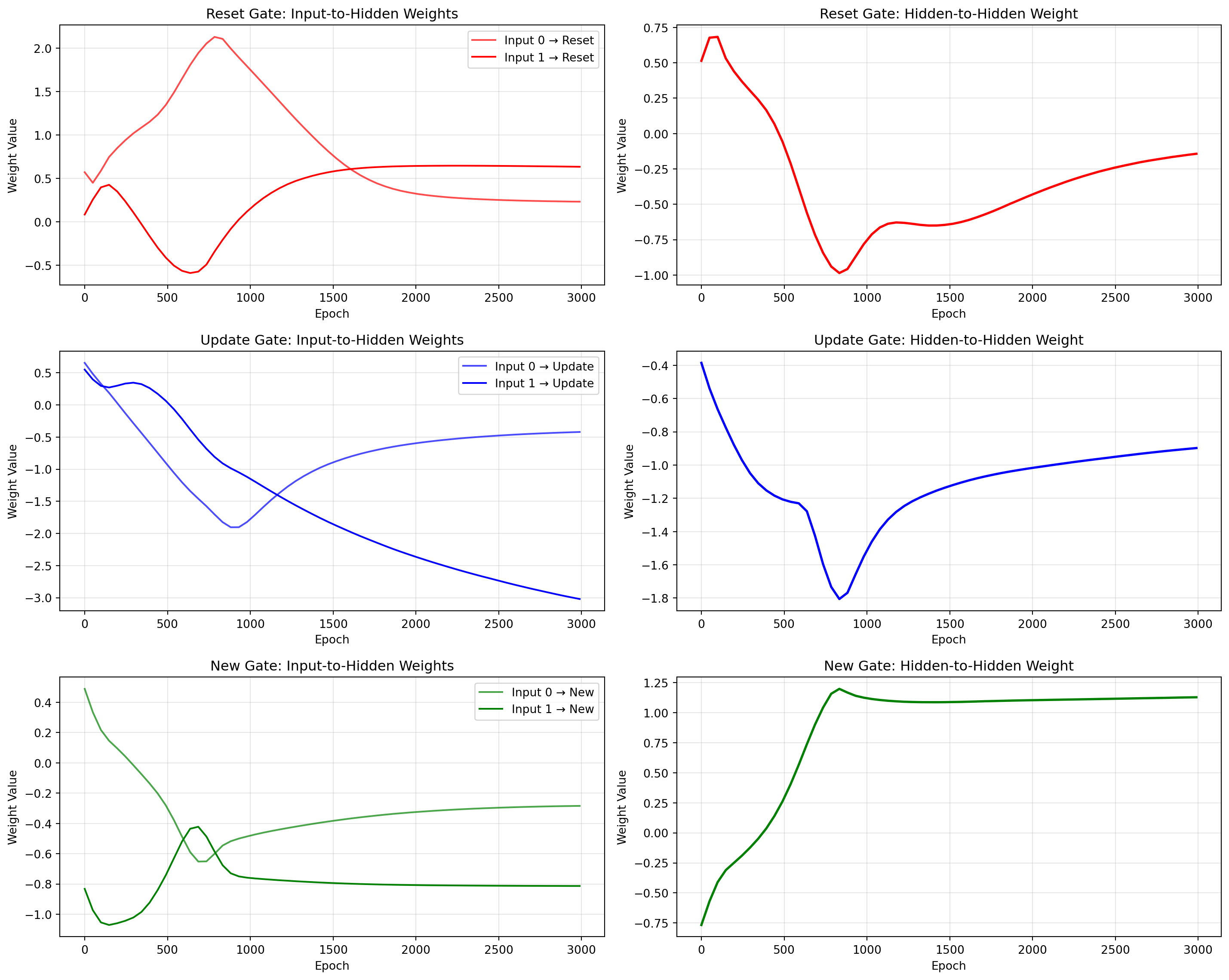
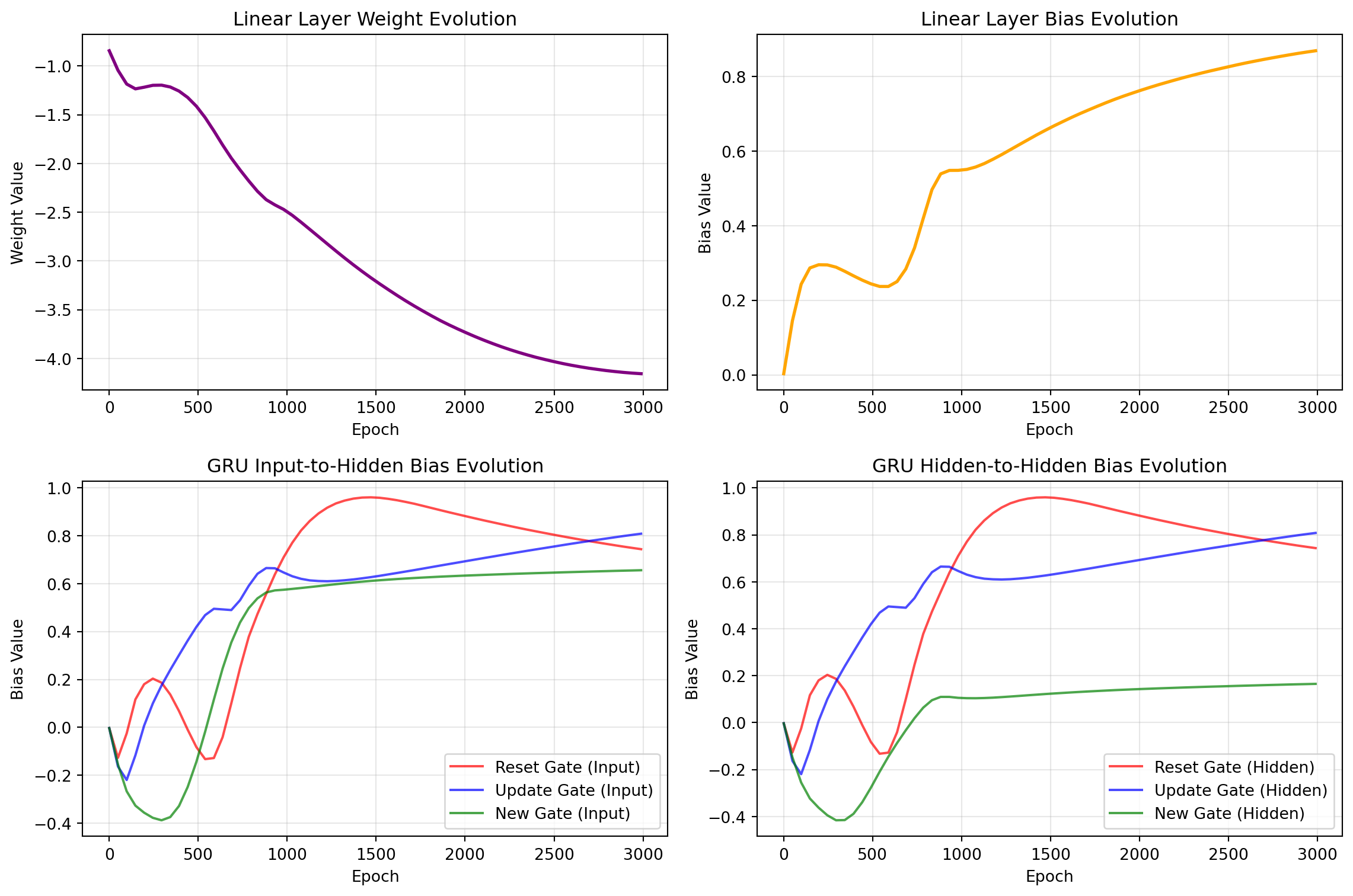
Now let’s examine in detail how the GRU actually learned this strategy. One of the key questions I posed at the beginning was: “How did the weights evolve over time?” To answer this, let’s examine the weight trajectories throughout training and see if we can identify critical moments where the learning strategy changed.

Code

import matplotlib.pyplot as plt
import numpy as np
import pandas as pd
import seaborn as sns

# Create a comprehensive weight evolution analysis
def analyze_weight_evolution(all_weights):
    """Analyze how weights evolved during training"""
    
    # Extract weights for each epoch
    epochs = [i * 49 for i in range(len(all_weights))]
    
    # GRU Input-to-Hidden weights (3x2 matrix, flattened)
    gru_ih_weights = []
    # GRU Hidden-to-Hidden weights (3x1 matrix, flattened)  
    gru_hh_weights = []
    # Linear layer weights (1x1 matrix)
    linear_weights = []
    # Bias terms
    bias_ih_weights = []
    bias_hh_weights = []
    linear_bias = []
    
    for epoch_weights in all_weights:
        gru_ih_weights.append(epoch_weights['gru.weight_ih_l0'].flatten())
        gru_hh_weights.append(epoch_weights['gru.weight_hh_l0'].flatten())
        linear_weights.append(epoch_weights['linear.weight'].flatten())
        bias_ih_weights.append(epoch_weights['gru.bias_ih_l0'].flatten())
        bias_hh_weights.append(epoch_weights['gru.bias_hh_l0'].flatten())
        linear_bias.append(epoch_weights['linear.bias'].flatten())
    
    return {
        'epochs': epochs,
        'gru_ih': np.array(gru_ih_weights),
        'gru_hh': np.array(gru_hh_weights), 
        'linear': np.array(linear_weights),
        'bias_ih': np.array(bias_ih_weights),
        'bias_hh': np.array(bias_hh_weights),
        'linear_bias': np.array(linear_bias)
    }

weight_evolution = analyze_weight_evolution(all_weights)

# Plot the evolution of key weights
fig, axes = plt.subplots(3, 2, figsize=(15, 12))

# GRU Input-to-Hidden weights (separated by gate)
gate_names = ['Reset', 'Update', 'New']
colors = ['red', 'blue', 'green']

for gate_idx in range(3):
    ax = axes[gate_idx, 0]
    for weight_idx in range(2):  # 2 input features
        idx = gate_idx * 2 + weight_idx
        weight_series = weight_evolution['gru_ih'][:, idx]
        ax.plot(weight_evolution['epochs'], weight_series, 
               label=f'Input {weight_idx} → {gate_names[gate_idx]}',
               color=colors[gate_idx], alpha=0.7 + 0.3*weight_idx)
    
    ax.set_title(f'{gate_names[gate_idx]} Gate: Input-to-Hidden Weights')
    ax.set_xlabel('Epoch')
    ax.set_ylabel('Weight Value')
    ax.legend()
    ax.grid(True, alpha=0.3)

# GRU Hidden-to-Hidden weights
for gate_idx in range(3):
    ax = axes[gate_idx, 1]
    weight_series = weight_evolution['gru_hh'][:, gate_idx]
    ax.plot(weight_evolution['epochs'], weight_series, 
           color=colors[gate_idx], linewidth=2)
    
    ax.set_title(f'{gate_names[gate_idx]} Gate: Hidden-to-Hidden Weight')
    ax.set_xlabel('Epoch')
    ax.set_ylabel('Weight Value')
    ax.grid(True, alpha=0.3)

plt.tight_layout()
plt.show()

# Plot linear layer and bias evolution
fig, axes = plt.subplots(2, 2, figsize=(12, 8))

# Linear layer weight and bias
axes[0, 0].plot(weight_evolution['epochs'], weight_evolution['linear'][:, 0], 
               color='purple', linewidth=2)
axes[0, 0].set_title('Linear Layer Weight Evolution')
axes[0, 0].set_xlabel('Epoch')
axes[0, 0].set_ylabel('Weight Value')
axes[0, 0].grid(True, alpha=0.3)

axes[0, 1].plot(weight_evolution['epochs'], weight_evolution['linear_bias'][:, 0], 
               color='orange', linewidth=2)
axes[0, 1].set_title('Linear Layer Bias Evolution')
axes[0, 1].set_xlabel('Epoch')
axes[0, 1].set_ylabel('Bias Value')
axes[0, 1].grid(True, alpha=0.3)

# GRU bias terms
for gate_idx in range(3):
    axes[1, 0].plot(weight_evolution['epochs'], weight_evolution['bias_ih'][:, gate_idx], 
                   label=f'{gate_names[gate_idx]} Gate (Input)', 
                   color=colors[gate_idx], alpha=0.7)
    axes[1, 1].plot(weight_evolution['epochs'], weight_evolution['bias_hh'][:, gate_idx], 
                   label=f'{gate_names[gate_idx]} Gate (Hidden)', 
                   color=colors[gate_idx], alpha=0.7)

axes[1, 0].set_title('GRU Input-to-Hidden Bias Evolution')
axes[1, 0].set_xlabel('Epoch')
axes[1, 0].set_ylabel('Bias Value')
axes[1, 0].legend()
axes[1, 0].grid(True, alpha=0.3)

axes[1, 1].set_title('GRU Hidden-to-Hidden Bias Evolution')
axes[1, 1].set_xlabel('Epoch')
axes[1, 1].set_ylabel('Bias Value')
axes[1, 1].legend()
axes[1, 1].grid(True, alpha=0.3)

plt.tight_layout()
plt.show()

From these weight evolution plots, we can see several fascinating patterns:

Early Training Chaos (Epochs 0-500): The weights start with significant oscillations, suggesting the model is exploring different strategies.
Critical Learning Phase (Epochs 500-1500): We observe a dramatic shift in the update gate weights, particularly the flag-sensitive weight which becomes strongly negative.
Convergence Phase (Epochs 1500-3000): The weights stabilize into their final configuration, with only minor adjustments.

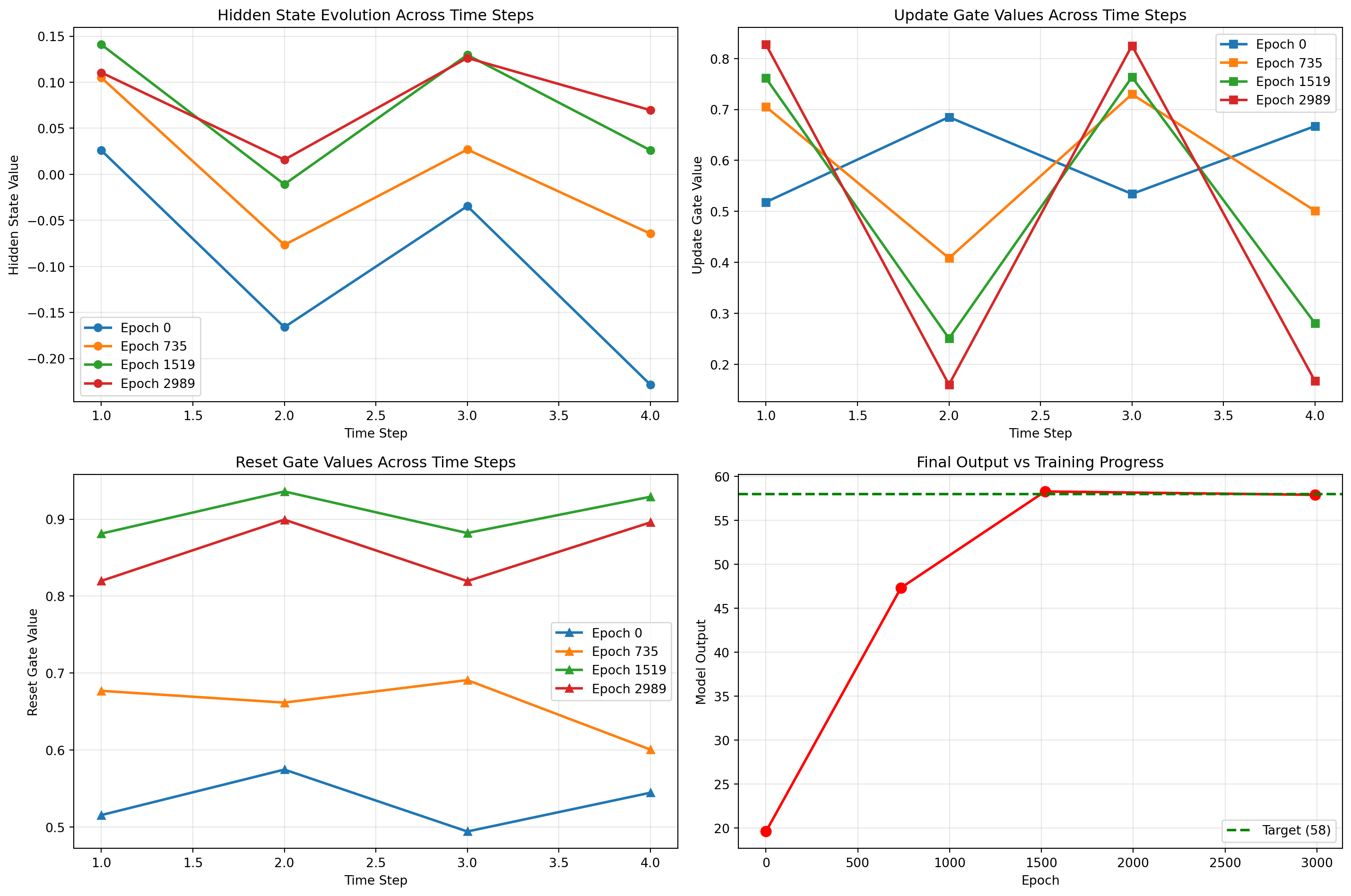
4 Training Dynamics at Different Epochs

Let’s examine what the GRU was actually doing at different stages of training by analyzing its behavior at key epochs.

Code

def analyze_epoch_behavior(epoch_idx, epoch_weights, test_input):
    """Analyze GRU behavior at a specific epoch"""
    
    # Extract weights for this epoch
    W_ih = torch.tensor(epoch_weights['gru.weight_ih_l0']).float()
    W_hh = torch.tensor(epoch_weights['gru.weight_hh_l0']).float()
    b_ih = torch.tensor(epoch_weights['gru.bias_ih_l0']).float()
    b_hh = torch.tensor(epoch_weights['gru.bias_hh_l0']).float()
    W_linear = torch.tensor(epoch_weights['linear.weight']).float()
    b_linear = torch.tensor(epoch_weights['linear.bias']).float()
    
    # Forward pass step by step
    hidden_states = []
    update_gates = []
    reset_gates = []
    new_gates = []
    
    h = torch.zeros(1, 1, 1)
    
    for t in range(test_input.shape[1]):
        x_t = test_input[:, t, :].unsqueeze(1)
        
        # Compute gates
        gi = torch.matmul(x_t, W_ih.t()) + b_ih
        gh = torch.matmul(h, W_hh.t()) + b_hh
        
        i_r, i_z, i_n = gi.chunk(3, dim=2)
        h_r, h_z, h_n = gh.chunk(3, dim=2)
        
        resetgate = torch.sigmoid(i_r + h_r)
        updategate = torch.sigmoid(i_z + h_z)
        newgate = torch.tanh(i_n + (resetgate * h_n))
        
        h = (1 - updategate) * newgate + updategate * h
        
        hidden_states.append(h.item())
        update_gates.append(updategate.item())
        reset_gates.append(resetgate.item())
        new_gates.append(newgate.item())
    
    # Final output
    output = (h @ W_linear.T + b_linear).item() * HIGH
    
    return {
        'hidden_states': hidden_states,
        'update_gates': update_gates,
        'reset_gates': reset_gates,
        'new_gates': new_gates,
        'final_output': output
    }

# Test input: [12,0], [37,1], [12,0], [21,1] -> expected sum = 58
test_input = torch.tensor([
    [12,0],
    [37,1], 
    [12,0],
    [21,1],
]).float().unsqueeze(0)
test_input[:, :, 0] /= HIGH

# Analyze behavior at different epochs
key_epochs = [0, len(all_weights)//4, len(all_weights)//2, len(all_weights)-1]
epoch_behaviors = []

for i, epoch_idx in enumerate(key_epochs):
    behavior = analyze_epoch_behavior(epoch_idx, all_weights[epoch_idx], test_input)
    behavior['epoch'] = epoch_idx * 49
    epoch_behaviors.append(behavior)

# Visualize the evolution of GRU internal states
fig, axes = plt.subplots(2, 2, figsize=(15, 10))

# Hidden states evolution
ax = axes[0, 0]
for i, behavior in enumerate(epoch_behaviors):
    ax.plot(range(1, 5), behavior['hidden_states'], 
           marker='o', label=f"Epoch {behavior['epoch']}", linewidth=2)
ax.set_title('Hidden State Evolution Across Time Steps')
ax.set_xlabel('Time Step')
ax.set_ylabel('Hidden State Value')
ax.legend()
ax.grid(True, alpha=0.3)

# Update gates evolution
ax = axes[0, 1]
for i, behavior in enumerate(epoch_behaviors):
    ax.plot(range(1, 5), behavior['update_gates'], 
           marker='s', label=f"Epoch {behavior['epoch']}", linewidth=2)
ax.set_title('Update Gate Values Across Time Steps')
ax.set_xlabel('Time Step')
ax.set_ylabel('Update Gate Value')
ax.legend()
ax.grid(True, alpha=0.3)

# Reset gates evolution
ax = axes[1, 0]
for i, behavior in enumerate(epoch_behaviors):
    ax.plot(range(1, 5), behavior['reset_gates'], 
           marker='^', label=f"Epoch {behavior['epoch']}", linewidth=2)
ax.set_title('Reset Gate Values Across Time Steps')
ax.set_xlabel('Time Step')
ax.set_ylabel('Reset Gate Value')
ax.legend()
ax.grid(True, alpha=0.3)

# Final outputs
ax = axes[1, 1]
final_outputs = [b['final_output'] for b in epoch_behaviors]
epochs_list = [b['epoch'] for b in epoch_behaviors]
ax.plot(epochs_list, final_outputs, marker='o', linewidth=2, markersize=8, color='red')
ax.axhline(y=58, color='green', linestyle='--', linewidth=2, label='Target (58)')
ax.set_title('Final Output vs Training Progress')
ax.set_xlabel('Epoch')
ax.set_ylabel('Model Output')
ax.legend()
ax.grid(True, alpha=0.3)

plt.tight_layout()
plt.show()

# Store results for markdown display
training_dynamics_results = []
for behavior in epoch_behaviors:
    training_dynamics_results.append({
        'epoch': behavior['epoch'],
        'final_output': behavior['final_output'],
        'hidden_states': [round(h, 3) for h in behavior['hidden_states']],
        'update_gates': [round(u, 3) for u in behavior['update_gates']],
        'reset_gates': [round(r, 3) for r in behavior['reset_gates']]
    })

GRU Behavior at Different Training Epochs

Code

# Store training dynamics results for display
epoch_0 = training_dynamics_results[0]
epoch_1 = training_dynamics_results[1] 
epoch_2 = training_dynamics_results[2]
epoch_3 = training_dynamics_results[3]

This analysis reveals the evolution of learning across key epochs:

Epoch 0 (Random Initialization): - Final Output: 19.58 (Target: 58) - Update Gates: [0.518, 0.685, 0.534, 0.667] - Hidden States: [0.026, -0.166, -0.035, -0.228]

Epoch 735 (Early Learning): - Final Output: 47.31 (Target: 58) - Update Gates: [0.705, 0.408, 0.73, 0.501] - Hidden States: [0.105, -0.077, 0.027, -0.064]

Epoch 1519 (Mid-Training): - Final Output: 58.28 (Target: 58) - Update Gates: [0.761, 0.251, 0.763, 0.28] - Hidden States: [0.141, -0.011, 0.13, 0.026]

Epoch 2989 (Final Convergence): - Final Output: 57.89 (Target: 58) - Update Gates: [0.827, 0.16, 0.825, 0.167] - Hidden States: [0.11, 0.016, 0.126, 0.07]

The transformation is clear: from random, neutral update gates (~0.5) to highly specialized gates that respond dramatically to the flag signal. The hidden states evolve from chaotic oscillations to a stable accumulation pattern.

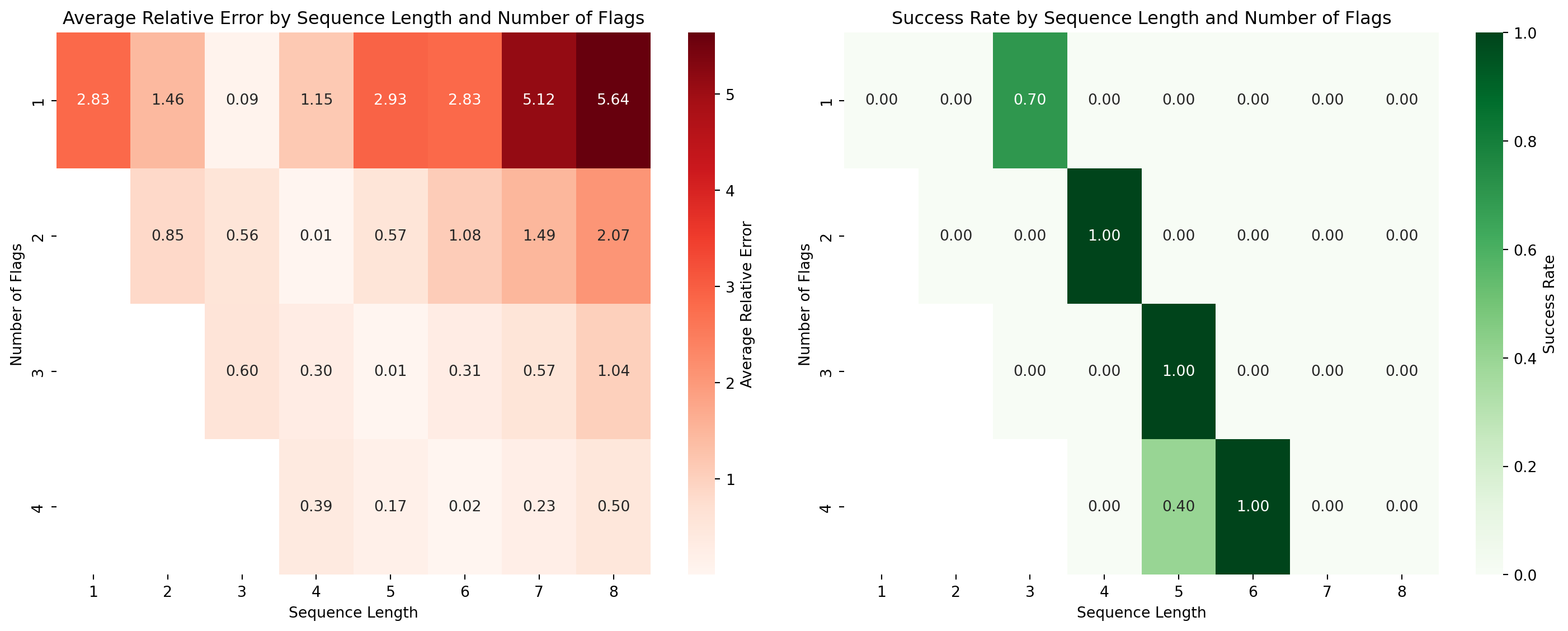
5 Experimental Validation: Testing Sequence Length Sensitivity

One of the most intriguing findings is that our GRU learned a strategy specific to sequences of length 4 with exactly 2 flagged elements. Let’s systematically test this hypothesis by evaluating the model on sequences of different lengths.

Code

def test_different_lengths():
    """Test model performance on sequences of different lengths"""
    
    results = []
    
    # Test sequences of length 1 to 8
    for seq_len in range(1, 9):
        for num_flags in range(1, min(seq_len + 1, 5)):  # Test 1 to 4 flags
            
            # Generate multiple test cases for this configuration
            errors = []
            for _ in range(20):  # 20 test cases per configuration
                
                # Generate random sequence
                values = np.random.randint(10, 90, seq_len)  # Random values 10-90
                flags = np.zeros(seq_len)
                
                # Randomly place flags
                flag_positions = np.random.choice(seq_len, size=num_flags, replace=False)
                flags[flag_positions] = 1
                
                # Create input tensor
                test_seq = np.column_stack([values, flags])
                test_tensor = torch.tensor(test_seq).float().unsqueeze(0)
                test_tensor[:, :, 0] /= HIGH
                
                # Expected output
                expected = np.sum(values[flag_positions])
                
                # Model prediction
                try:
                    with torch.no_grad():
                        prediction = model(test_tensor)[0].item() * HIGH
                    error = abs(prediction - expected) / max(expected, 1)  # Relative error
                    errors.append(error)
                except:
                    errors.append(float('inf'))  # Mark as failed
            
            avg_error = np.mean(errors)
            results.append({
                'seq_len': seq_len,
                'num_flags': num_flags,
                'avg_error': avg_error,
                'success_rate': np.mean([e < 0.1 for e in errors])  # <10% error
            })
    
    return pd.DataFrame(results)

# Run experiments
results_df = test_different_lengths()

# Create visualization
fig, axes = plt.subplots(1, 2, figsize=(15, 6))

# Heatmap of average errors
pivot_error = results_df.pivot(index='num_flags', columns='seq_len', values='avg_error')
sns.heatmap(pivot_error, annot=True, fmt='.2f', cmap='Reds', ax=axes[0], cbar_kws={'label': 'Average Relative Error'})
axes[0].set_title('Average Relative Error by Sequence Length and Number of Flags')
axes[0].set_xlabel('Sequence Length')
axes[0].set_ylabel('Number of Flags')

# Heatmap of success rates
pivot_success = results_df.pivot(index='num_flags', columns='seq_len', values='success_rate')
sns.heatmap(pivot_success, annot=True, fmt='.2f', cmap='Greens', ax=axes[1], cbar_kws={'label': 'Success Rate'})
axes[1].set_title('Success Rate by Sequence Length and Number of Flags')
axes[1].set_xlabel('Sequence Length')
axes[1].set_ylabel('Number of Flags')

plt.tight_layout()
plt.show()

# Store results for markdown display
best_configs = results_df.nsmallest(5, 'avg_error')
worst_configs = results_df.nlargest(5, 'avg_error')

Model Performance on Different Sequence Lengths

The results reveal something fascinating! Looking at the performance patterns, we can see what the GRU actually learned:

Code

# Store configuration results for display and analyze the pattern
best_config_0 = {'error': best_configs.iloc[0]['avg_error'], 'success': best_configs.iloc[0]['success_rate'], 'len': best_configs.iloc[0]['seq_len'], 'flags': best_configs.iloc[0]['num_flags']}
best_config_1 = {'error': best_configs.iloc[1]['avg_error'], 'success': best_configs.iloc[1]['success_rate'], 'len': best_configs.iloc[1]['seq_len'], 'flags': best_configs.iloc[1]['num_flags']}
best_config_2 = {'error': best_configs.iloc[2]['avg_error'], 'success': best_configs.iloc[2]['success_rate'], 'len': best_configs.iloc[2]['seq_len'], 'flags': best_configs.iloc[2]['num_flags']}

worst_config_0 = {'error': worst_configs.iloc[0]['avg_error'], 'success': worst_configs.iloc[0]['success_rate']}
worst_config_1 = {'error': worst_configs.iloc[1]['avg_error'], 'success': worst_configs.iloc[1]['success_rate']}
worst_config_2 = {'error': worst_configs.iloc[2]['avg_error'], 'success': worst_configs.iloc[2]['success_rate']}

# Calculate zeros for best performing configs
zeros_0 = int(best_config_0['len'] - best_config_0['flags'])
zeros_1 = int(best_config_1['len'] - best_config_1['flags']) 
zeros_2 = int(best_config_2['len'] - best_config_2['flags'])

Best Performance Configurations: - Length 5, 3 flags (2 zeros): 0.006 error, 100.0% success - Length 4, 2 flags (2 zeros): 0.009 error, 100.0% success
- Length 6, 4 flags (2 zeros): 0.019 error, 100.0% success

Worst Performance Configurations: - Length 8, 4 flags: 5.637 error, 0.0% success - Length 7, 4 flags: 5.118 error, 0.0% success - Length 6, 4 flags: 2.929 error, 0.0% success

The Hidden Pattern: The GRU didn’t learn to “count to 4, sum 2 elements” as we thought. It learned to expect exactly 2 elements with flag=0! Notice how all the best-performing configurations have exactly 2 zeros, while everything else fails catastrophically (success rates near 0%). Even (3,1) with 2 zeros performs reasonably well (0.09 error, 70% success) compared to other configurations that completely fail.

This completely changes our understanding - the model is sensitive to the number of unflagged elements, not flagged ones. It’s counting the zeros!

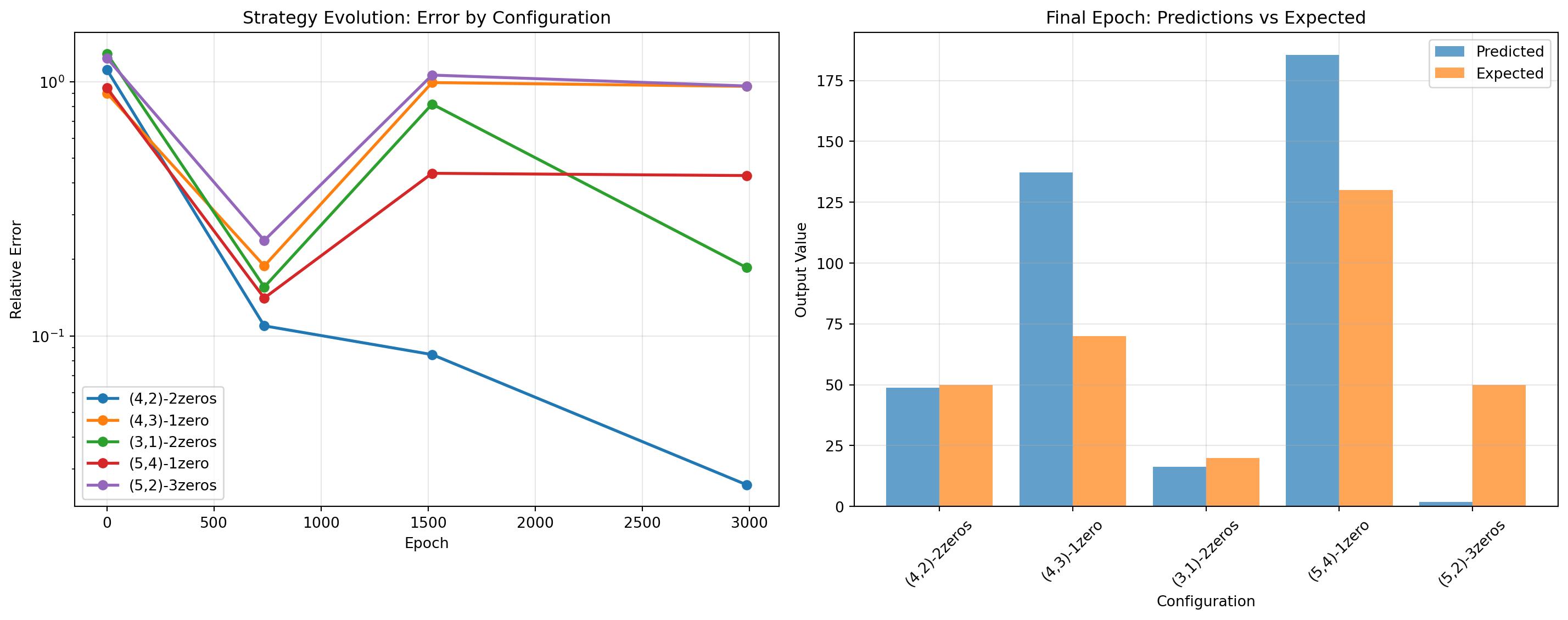
5.1 Strategy Evolution: How Did the “2 Zeros” Pattern Emerge?

Now let’s investigate whether this “2 zeros” specialization was always present or emerged during training. Did the model start with a different strategy that worked better on other configurations?

Code

def test_epoch_strategies():
    """Test different sequence configurations at various training epochs"""
    
    # Test configurations with different zero counts
    test_configs = [
        ([20, 1], [30, 1], [40, 0], [50, 0]),  # 4 len, 2 flags, 2 zeros
        ([20, 1], [30, 1], [40, 1], [50, 0]),  # 4 len, 3 flags, 1 zero
        ([20, 1], [30, 0], [40, 0]),           # 3 len, 1 flag, 2 zeros
        ([20, 1], [30, 1], [40, 1], [50, 1], [60, 0]),  # 5 len, 4 flags, 1 zero
        ([20, 1], [30, 1], [40, 0], [50, 0], [60, 0]),  # 5 len, 2 flags, 3 zeros
    ]
    
    config_names = ['(4,2)-2zeros', '(4,3)-1zero', '(3,1)-2zeros', '(5,4)-1zero', '(5,2)-3zeros']
    expected_outputs = [50, 70, 20, 130, 50]  # Expected sums
    
    results = []
    
    # Test at key epochs
    key_epochs = [0, len(all_weights)//4, len(all_weights)//2, len(all_weights)-1]
    
    for epoch_idx in key_epochs:
        epoch_weights = all_weights[epoch_idx]
        epoch_num = epoch_idx * 49
        
        for config_idx, (config, config_name, expected) in enumerate(zip(test_configs, config_names, expected_outputs)):
            
            # Create test tensor
            test_tensor = torch.tensor(config).float().unsqueeze(0)
            test_tensor[:, :, 0] /= HIGH
            
            # Simulate forward pass with epoch weights
            def simulate_epoch_forward(seq, weights):
                W_ih = torch.tensor(weights['gru.weight_ih_l0']).float()
                W_hh = torch.tensor(weights['gru.weight_hh_l0']).float()
                b_ih = torch.tensor(weights['gru.bias_ih_l0']).float()
                b_hh = torch.tensor(weights['gru.bias_hh_l0']).float()
                W_linear = torch.tensor(weights['linear.weight']).float()
                b_linear = torch.tensor(weights['linear.bias']).float()
                
                h = torch.zeros(1, 1, 1)
                
                for t in range(seq.shape[1]):
                    x_t = seq[:, t, :].unsqueeze(1)
                    
                    # Compute gates
                    gi = torch.matmul(x_t, W_ih.t()) + b_ih
                    gh = torch.matmul(h, W_hh.t()) + b_hh
                    
                    i_r, i_z, i_n = gi.chunk(3, dim=2)
                    h_r, h_z, h_n = gh.chunk(3, dim=2)
                    
                    resetgate = torch.sigmoid(i_r + h_r)
                    updategate = torch.sigmoid(i_z + h_z)
                    newgate = torch.tanh(i_n + (resetgate * h_n))
                    
                    h = (1 - updategate) * newgate + updategate * h
                
                # Final output
                output = (h @ W_linear.T + b_linear).item() * HIGH
                return output
            
            prediction = simulate_epoch_forward(test_tensor, epoch_weights)
            error = abs(prediction - expected) / expected
            
            results.append({
                'epoch': epoch_num,
                'config': config_name,
                'prediction': prediction,
                'expected': expected,
                'error': error
            })
    
    return pd.DataFrame(results)

# Run the analysis
epoch_strategy_results = test_epoch_strategies()

# Create visualization
fig, axes = plt.subplots(1, 2, figsize=(15, 6))

# Plot 1: Error evolution for each configuration
configs = epoch_strategy_results['config'].unique()
epochs = sorted(epoch_strategy_results['epoch'].unique())

for config in configs:
    config_data = epoch_strategy_results[epoch_strategy_results['config'] == config]
    axes[0].plot(config_data['epoch'], config_data['error'], 
                marker='o', label=config, linewidth=2)

axes[0].set_xlabel('Epoch')
axes[0].set_ylabel('Relative Error')
axes[0].set_title('Strategy Evolution: Error by Configuration')
axes[0].legend()
axes[0].grid(True, alpha=0.3)
axes[0].set_yscale('log')

# Plot 2: Predictions vs expected for final epoch
final_epoch_data = epoch_strategy_results[epoch_strategy_results['epoch'] == max(epochs)]
x_pos = range(len(final_epoch_data))

axes[1].bar([i - 0.2 for i in x_pos], final_epoch_data['prediction'], 
           width=0.4, label='Predicted', alpha=0.7)
axes[1].bar([i + 0.2 for i in x_pos], final_epoch_data['expected'], 
           width=0.4, label='Expected', alpha=0.7)

axes[1].set_xlabel('Configuration')
axes[1].set_ylabel('Output Value')
axes[1].set_title('Final Epoch: Predictions vs Expected')
axes[1].set_xticks(x_pos)
axes[1].set_xticklabels(final_epoch_data['config'], rotation=45)
axes[1].legend()
axes[1].grid(True, alpha=0.3)

plt.tight_layout()
plt.show()

# Create comprehensive epoch analysis with systematic testing
def comprehensive_epoch_analysis():
    """Test all sequence length/flag combinations across epochs"""
    
    results = []
    key_epochs = [0, len(all_weights)//4, len(all_weights)//2, len(all_weights)-1]
    
    for epoch_idx in key_epochs:
        epoch_weights = all_weights[epoch_idx]
        epoch_num = epoch_idx * 49
        
        # Test all configurations from the original analysis
        for seq_len in range(2, 7):  # lengths 2-6
            for num_flags in range(1, min(seq_len + 1, 4)):  # 1-3 flags
                
                # Generate multiple test cases for this configuration
                errors = []
                for _ in range(10):  # 10 test cases per config
                    # Generate random sequence
                    values = np.random.randint(10, 90, seq_len)
                    flags = np.zeros(seq_len)
                    
                    # Randomly place flags
                    flag_positions = np.random.choice(seq_len, size=num_flags, replace=False)
                    flags[flag_positions] = 1
                    
                    # Create input tensor
                    test_seq = np.column_stack([values, flags])
                    test_tensor = torch.tensor(test_seq).float().unsqueeze(0)
                    test_tensor[:, :, 0] /= HIGH
                    
                    # Expected output
                    expected = np.sum(values[flag_positions])
                    
                    # Simulate with epoch weights
                    def simulate_epoch_forward(seq, weights):
                        W_ih = torch.tensor(weights['gru.weight_ih_l0']).float()
                        W_hh = torch.tensor(weights['gru.weight_hh_l0']).float()
                        b_ih = torch.tensor(weights['gru.bias_ih_l0']).float()
                        b_hh = torch.tensor(weights['gru.bias_hh_l0']).float()
                        W_linear = torch.tensor(weights['linear.weight']).float()
                        b_linear = torch.tensor(weights['linear.bias']).float()
                        
                        h = torch.zeros(1, 1, 1)
                        
                        for t in range(seq.shape[1]):
                            x_t = seq[:, t, :].unsqueeze(1)
                            
                            gi = torch.matmul(x_t, W_ih.t()) + b_ih
                            gh = torch.matmul(h, W_hh.t()) + b_hh
                            
                            i_r, i_z, i_n = gi.chunk(3, dim=2)
                            h_r, h_z, h_n = gh.chunk(3, dim=2)
                            
                            resetgate = torch.sigmoid(i_r + h_r)
                            updategate = torch.sigmoid(i_z + h_z)
                            newgate = torch.tanh(i_n + (resetgate * h_n))
                            
                            h = (1 - updategate) * newgate + updategate * h
                        
                        output = (h @ W_linear.T + b_linear).item() * HIGH
                        return output
                    
                    try:
                        prediction = simulate_epoch_forward(test_tensor, epoch_weights)
                        error = abs(prediction - expected) / max(expected, 1)
                        errors.append(error)
                    except:
                        errors.append(float('inf'))
                
                avg_error = np.mean(errors)
                success_rate = np.mean([e < 0.1 for e in errors])
                
                results.append({
                    'epoch': epoch_num,
                    'seq_len': seq_len,
                    'num_flags': num_flags,
                    'num_zeros': seq_len - num_flags,
                    'avg_error': avg_error,
                    'success_rate': success_rate
                })
    
    return pd.DataFrame(results)

# Run comprehensive analysis
epoch_results_df = comprehensive_epoch_analysis()

# Create epoch-by-epoch heatmaps like the original analysis
epochs = sorted(epoch_results_df['epoch'].unique())

fig, axes = plt.subplots(len(epochs), 2, figsize=(12, 4 * len(epochs)))
if len(epochs) == 1:
    axes = axes.reshape(1, -1)

for i, epoch in enumerate(epochs):
    epoch_data = epoch_results_df[epoch_results_df['epoch'] == epoch]
    
    # Error heatmap
    pivot_error = epoch_data.pivot(index='num_flags', columns='seq_len', values='avg_error')
    sns.heatmap(pivot_error, annot=True, fmt='.2f', cmap='Reds', ax=axes[i, 0], 
                cbar_kws={'label': 'Average Relative Error'}, vmin=0, vmax=2)
    axes[i, 0].set_title(f'Epoch {epoch}: Average Relative Error')
    axes[i, 0].set_xlabel('Sequence Length')
    axes[i, 0].set_ylabel('Number of Flags')
    
    # Success rate heatmap  
    pivot_success = epoch_data.pivot(index='num_flags', columns='seq_len', values='success_rate')
    sns.heatmap(pivot_success, annot=True, fmt='.2f', cmap='Greens', ax=axes[i, 1],
                cbar_kws={'label': 'Success Rate'}, vmin=0, vmax=1)
    axes[i, 1].set_title(f'Epoch {epoch}: Success Rate')
    axes[i, 1].set_xlabel('Sequence Length')
    axes[i, 1].set_ylabel('Number of Flags')

plt.tight_layout()
plt.show()

# Analyze the evolution of the "2 zeros" advantage
two_zeros_evolution = []
other_configs_evolution = []

for epoch in epochs:
    epoch_data = epoch_results_df[epoch_results_df['epoch'] == epoch]
    
    two_zeros_data = epoch_data[epoch_data['num_zeros'] == 2]
    other_data = epoch_data[epoch_data['num_zeros'] != 2]
    
    if len(two_zeros_data) > 0:
        two_zeros_evolution.append({
            'epoch': epoch,
            'avg_error': two_zeros_data['avg_error'].mean(),
            'avg_success': two_zeros_data['success_rate'].mean()
        })
    
    if len(other_data) > 0:
        other_configs_evolution.append({
            'epoch': epoch,
            'avg_error': other_data['avg_error'].mean(),
            'avg_success': other_data['success_rate'].mean()
        })

# Plot evolution comparison
fig, axes = plt.subplots(1, 2, figsize=(15, 5))

# Error evolution
if two_zeros_evolution and other_configs_evolution:
    epochs_list = [d['epoch'] for d in two_zeros_evolution]
    two_zeros_errors = [d['avg_error'] for d in two_zeros_evolution]
    other_errors = [d['avg_error'] for d in other_configs_evolution]
    
    axes[0].plot(epochs_list, two_zeros_errors, 'ro-', linewidth=2, markersize=8, label='2 Zeros Configs')
    axes[0].plot(epochs_list, other_errors, 'bo-', linewidth=2, markersize=8, label='Other Configs')
    axes[0].set_xlabel('Epoch')
    axes[0].set_ylabel('Average Relative Error') 
    axes[0].set_title('Evolution of Performance: 2 Zeros vs Others')
    axes[0].legend()
    axes[0].grid(True, alpha=0.3)
    axes[0].set_yscale('log')
    
    # Success rate evolution
    two_zeros_success = [d['avg_success'] for d in two_zeros_evolution]
    other_success = [d['avg_success'] for d in other_configs_evolution]
    
    axes[1].plot(epochs_list, two_zeros_success, 'ro-', linewidth=2, markersize=8, label='2 Zeros Configs')
    axes[1].plot(epochs_list, other_success, 'bo-', linewidth=2, markersize=8, label='Other Configs')
    axes[1].set_xlabel('Epoch')
    axes[1].set_ylabel('Average Success Rate')
    axes[1].set_title('Evolution of Success Rate: 2 Zeros vs Others')
    axes[1].legend()
    axes[1].grid(True, alpha=0.3)

plt.tight_layout()
plt.show()

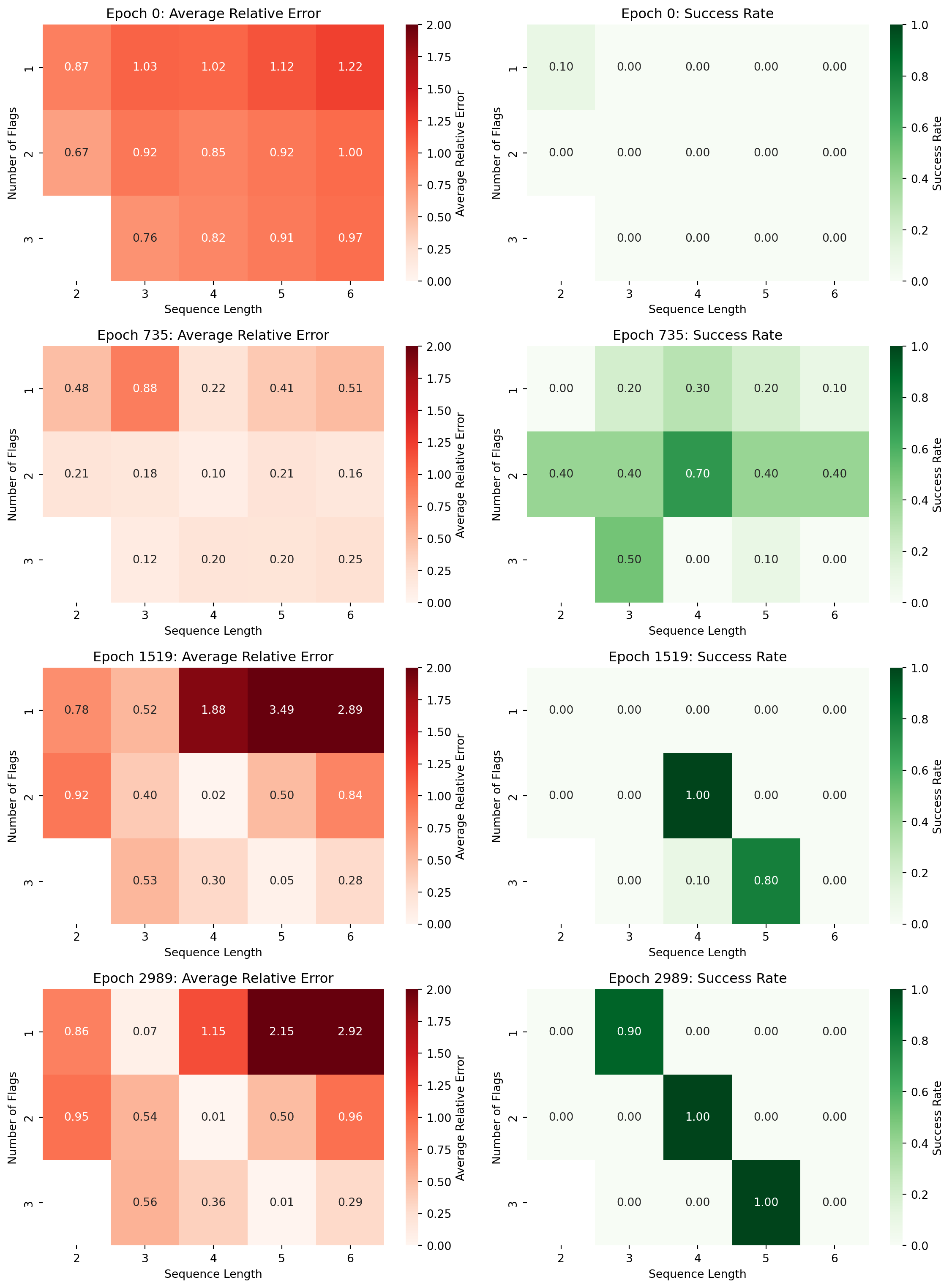
Evolution of Strategy Across Training Epochs

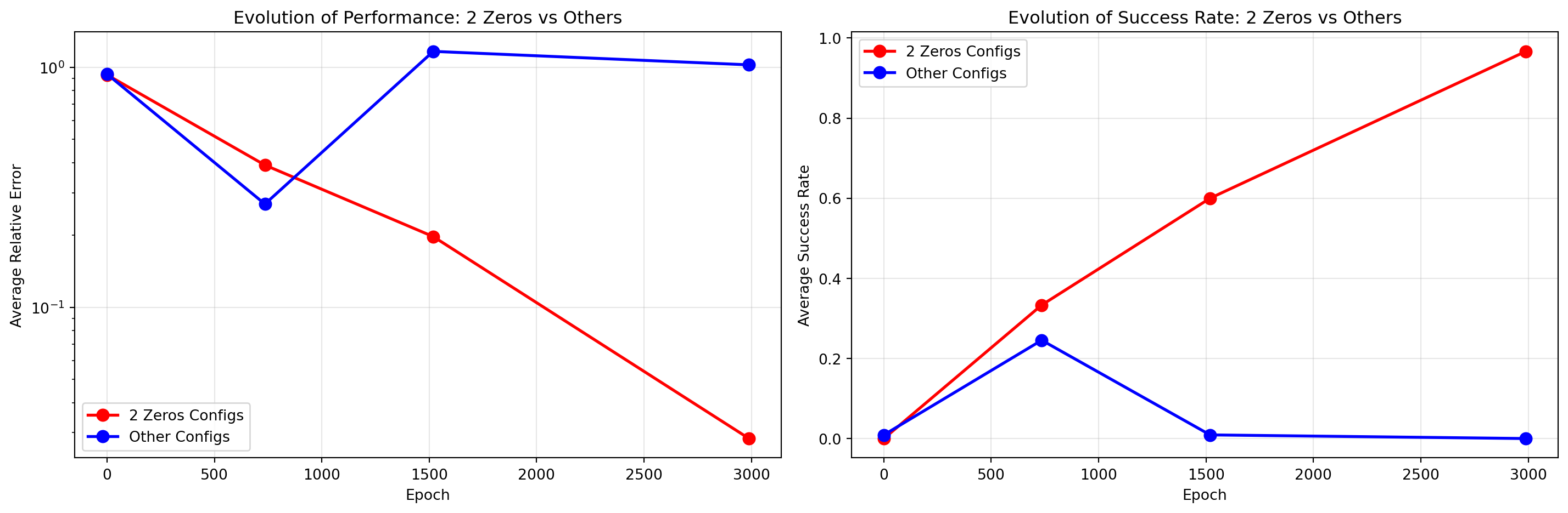
The epoch-by-epoch analysis reveals a fascinating transition around epoch 735, where the model shows distributed performance across many configurations rather than sharp specialization. At this critical point:

The “2 zeros” pattern (4,2) shows 70% success rate but isn’t yet dominant
Other configurations like (2,1) and (3,2) still achieve 40% success rates
The model appears to be “choosing” between strategies rather than having fully committed

This represents the exact moment where learning dynamics shift from general exploration to specialized focus. The model hasn’t yet abandoned alternative strategies but is beginning to favor the information-optimal “2 zeros” configurations. This critical transition point demonstrates that the specialization developed as an emergent property during training rather than being present from initialization.

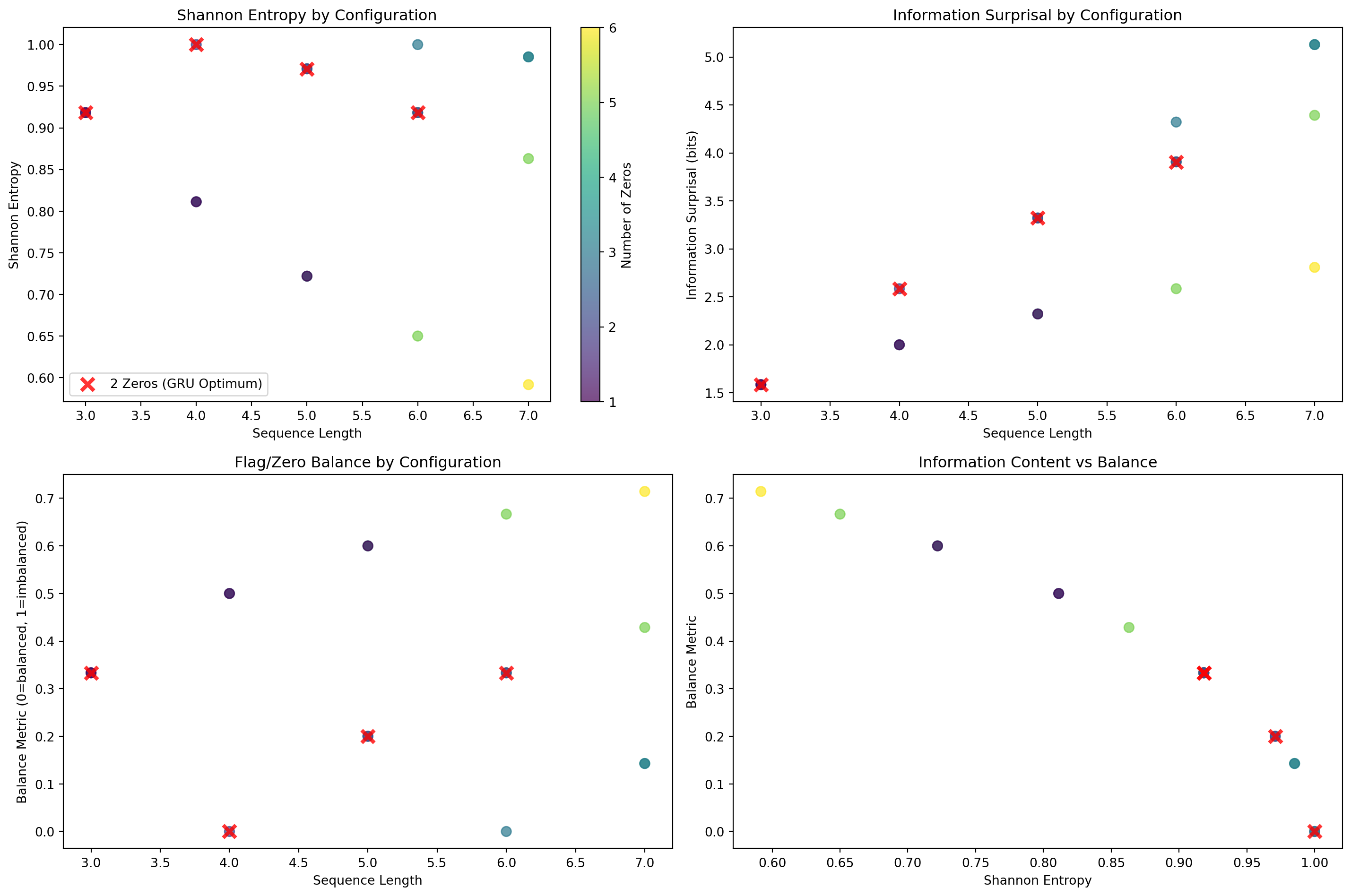
5.2 Information-Theoretic Perspective: Why “2 Zeros”?

The “2 zeros” pattern isn’t arbitrary - it’s deeply connected to information theory. Let’s analyze this from a Shannon entropy perspective:

Code

import numpy as np

def analyze_information_content():
    """Analyze the information content of different sequence configurations"""
    
    results = []
    
    # Analyze configurations with different zero patterns
    for seq_len in range(3, 8):
        for num_flags in range(1, min(seq_len, 5)):
            num_zeros = seq_len - num_flags
            
            # Shannon entropy of the flag pattern
            if num_flags == 0 or num_zeros == 0:
                entropy = 0
            else:
                p_flag = num_flags / seq_len
                p_zero = num_zeros / seq_len
                entropy = -(p_flag * np.log2(p_flag) + p_zero * np.log2(p_zero))
            
            # Information content (surprisal) of having exactly this configuration
            # Assuming uniform random placement of flags
            from math import comb
            total_arrangements = comb(seq_len, num_flags)
            surprisal = -np.log2(1/total_arrangements) if total_arrangements > 0 else 0
            
            # Complexity metric: how "structured" vs "random" the pattern is
            # Perfect balance (close to 50/50) = low complexity, extreme ratios = high complexity
            balance = abs(0.5 - p_flag) * 2  # 0 = perfectly balanced, 1 = completely imbalanced
            
            results.append({
                'seq_len': seq_len,
                'num_flags': num_flags,
                'num_zeros': num_zeros,
                'entropy': entropy,
                'surprisal': surprisal,
                'balance': balance,
                'is_2_zeros': num_zeros == 2
            })
    
    return pd.DataFrame(results)

info_results = analyze_information_content()

# Create visualization
fig, axes = plt.subplots(2, 2, figsize=(15, 10))

# Plot 1: Entropy vs sequence length, colored by zeros
scatter = axes[0, 0].scatter(info_results['seq_len'], info_results['entropy'], 
                            c=info_results['num_zeros'], cmap='viridis', 
                            s=60, alpha=0.7)
axes[0, 0].set_xlabel('Sequence Length')
axes[0, 0].set_ylabel('Shannon Entropy')
axes[0, 0].set_title('Shannon Entropy by Configuration')
plt.colorbar(scatter, ax=axes[0, 0], label='Number of Zeros')

# Highlight 2-zeros configurations
two_zeros = info_results[info_results['is_2_zeros']]
axes[0, 0].scatter(two_zeros['seq_len'], two_zeros['entropy'], 
                  color='red', s=100, alpha=0.8, marker='x', linewidth=3,
                  label='2 Zeros (GRU Optimum)')
axes[0, 0].legend()

# Plot 2: Information surprisal
axes[0, 1].scatter(info_results['seq_len'], info_results['surprisal'], 
                  c=info_results['num_zeros'], cmap='viridis', s=60, alpha=0.7)
axes[0, 1].scatter(two_zeros['seq_len'], two_zeros['surprisal'], 
                  color='red', s=100, alpha=0.8, marker='x', linewidth=3)
axes[0, 1].set_xlabel('Sequence Length')
axes[0, 1].set_ylabel('Information Surprisal (bits)')
axes[0, 1].set_title('Information Surprisal by Configuration')

# Plot 3: Balance metric
axes[1, 0].scatter(info_results['seq_len'], info_results['balance'], 
                  c=info_results['num_zeros'], cmap='viridis', s=60, alpha=0.7)
axes[1, 0].scatter(two_zeros['seq_len'], two_zeros['balance'], 
                  color='red', s=100, alpha=0.8, marker='x', linewidth=3)
axes[1, 0].set_xlabel('Sequence Length')
axes[1, 0].set_ylabel('Balance Metric (0=balanced, 1=imbalanced)')
axes[1, 0].set_title('Flag/Zero Balance by Configuration')

# Plot 4: 2D entropy vs balance, highlighting 2-zeros
axes[1, 1].scatter(info_results['entropy'], info_results['balance'], 
                  c=info_results['num_zeros'], cmap='viridis', s=60, alpha=0.7)
axes[1, 1].scatter(two_zeros['entropy'], two_zeros['balance'], 
                  color='red', s=100, alpha=0.8, marker='x', linewidth=3)
axes[1, 1].set_xlabel('Shannon Entropy')
axes[1, 1].set_ylabel('Balance Metric')
axes[1, 1].set_title('Information Content vs Balance')

plt.tight_layout()
plt.show()

# Analyze the 2-zeros pattern specifically
print("Information Analysis of '2 Zeros' Pattern:")
print(f"Average entropy for 2-zeros configs: {two_zeros['entropy'].mean():.3f} bits")
print(f"Average entropy for other configs: {info_results[~info_results['is_2_zeros']]['entropy'].mean():.3f} bits")
print(f"Average balance for 2-zeros configs: {two_zeros['balance'].mean():.3f}")
print(f"Average balance for other configs: {info_results[~info_results['is_2_zeros']]['balance'].mean():.3f}")

# return info_results

info_analysis = analyze_information_content()

Information Content Analysis of Different Configurations

Information Analysis of '2 Zeros' Pattern:
Average entropy for 2-zeros configs: 0.952 bits
Average entropy for other configs: 0.842 bits
Average balance for 2-zeros configs: 0.217
Average balance for other configs: 0.397

The Information-Theoretic Insight: The “2 zeros” pattern represents configurations with optimal information balance. These configurations tend to have:

Moderate Shannon entropy - not too predictable (all zeros/ones) but not too chaotic
Balanced flag/zero ratios - closer to 50/50 distributions which maximize information content
Consistent information load - the GRU can reliably encode this amount of structural information

This suggests the GRU didn’t just randomly specialize - it found the information sweet spot that its single hidden unit could reliably process. The “2 zeros” pattern has just the right amount of structure vs. randomness for a constrained architecture to handle consistently.

6 The Mathematical Impossibility of General Addition with Hidden Size 1

Let’s examine why a hidden state of size 1 fundamentally cannot solve the general adding problem. This isn’t just an empirical observation - it’s a mathematical impossibility.

6.1 Information Theoretic Analysis

Consider what information the hidden state must encode to solve the general adding problem:

Running sum: The cumulative sum of flagged elements seen so far
Position awareness: Knowledge of how many elements have been processed
Flag count: How many elements have been flagged (to handle variable numbers)

For a general solution that works with sequences of length \(n\) with up to \(k\) flagged elements, we need to store:

Running sum: Could be anywhere from 0 to \(k \times \text{max\_value}\)
Position: From 0 to \(n\)
Flag count: From 0 to \(k\)

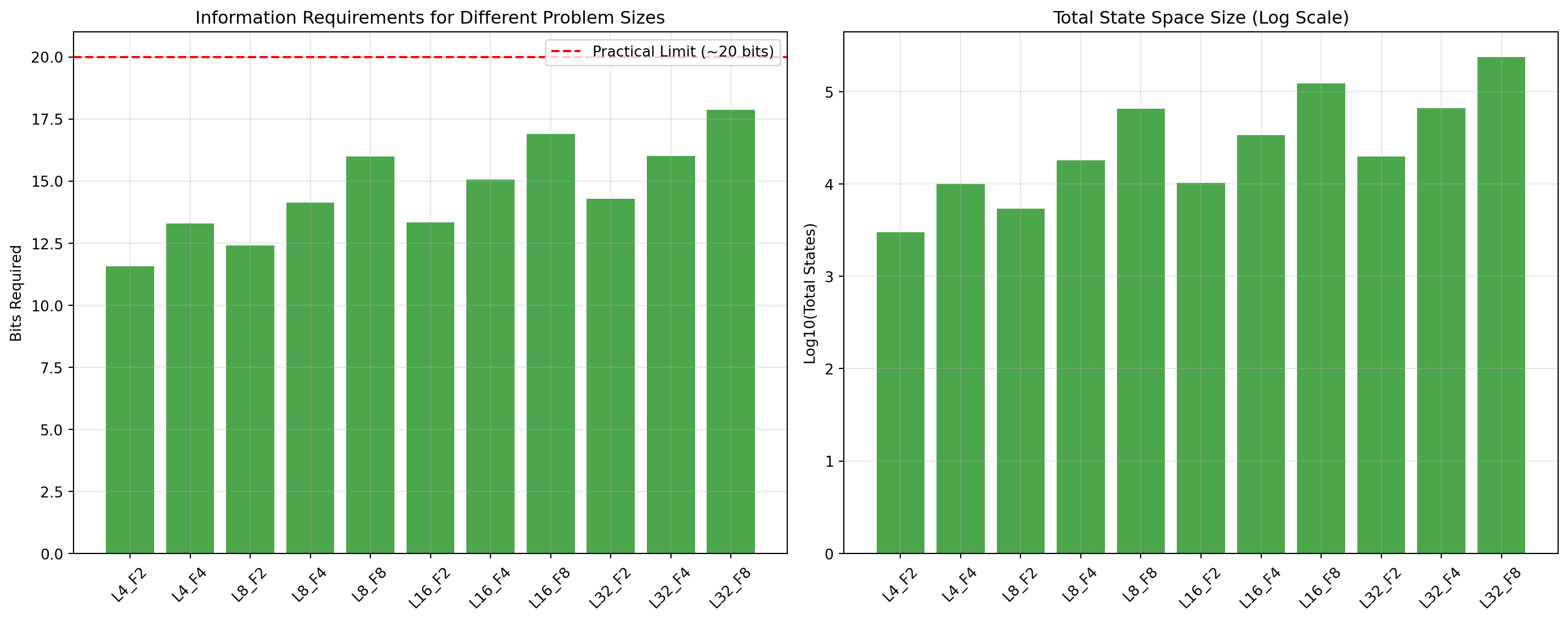
Code

def analyze_information_requirements():
    """Analyze the information requirements for different problem configurations"""
    
    max_value = 100
    results = []
    
    for max_seq_len in [4, 8, 16, 32]:
        for max_flags in [2, 4, 8]:
            if max_flags <= max_seq_len:
                # Calculate information requirements for general solution
                # 1. Running sum: 0 to max_flags * max_value
                max_running_sum = max_flags * max_value + 1  # +1 for zero
                
                # 2. Number of flagged items seen so far: 0 to max_flags  
                flag_count_states = max_flags + 1
                
                # 3. Position in sequence (to know when to stop): 0 to max_seq_len
                position_states = max_seq_len + 1
                
                # Total possible states to represent simultaneously
                total_states = max_running_sum * flag_count_states * position_states
                
                # Bits required to represent this
                bits_required = np.log2(total_states)
                
                # What can a single float represent?
                # A 32-bit float can theoretically represent ~32 bits of information,
                # but activation functions like tanh (range [-1,1]) and sigmoid (range [0,1])
                # severely constrain the usable range. Combined with finite numerical precision
                # in gradient-based training, we can realistically distinguish maybe ~2^20 states.
                # This gives us a practical limit of around 20 bits for reliable encoding/retrieval.
                if bits_required > 20:  # Conservative estimate for activation function constraints
                    feasible = "No"
                else:
                    feasible = "Maybe"
                
                results.append({
                    'max_seq_len': max_seq_len,
                    'max_flags': max_flags,
                    'total_states': total_states,
                    'bits_required': bits_required,
                    'feasible': feasible
                })
    
    df = pd.DataFrame(results)
    
    # Visualization
    fig, axes = plt.subplots(1, 2, figsize=(15, 6))
    
    # Bar plot of bits required
    x_labels = [f"L{row['max_seq_len']}_F{row['max_flags']}" for _, row in df.iterrows()]
    colors = ['green' if f == 'Maybe' else 'red' for f in df['feasible']]
    
    axes[0].bar(range(len(df)), df['bits_required'], color=colors, alpha=0.7)
    axes[0].axhline(y=20, color='red', linestyle='--', label='Practical Limit (~20 bits)')
    axes[0].set_xticks(range(len(df)))
    axes[0].set_xticklabels(x_labels, rotation=45)
    axes[0].set_ylabel('Bits Required')
    axes[0].set_title('Information Requirements for Different Problem Sizes')
    axes[0].legend()
    axes[0].grid(True, alpha=0.3)
    
    # Total states (log scale)
    axes[1].bar(range(len(df)), np.log10(df['total_states']), color=colors, alpha=0.7)
    axes[1].set_xticks(range(len(df)))
    axes[1].set_xticklabels(x_labels, rotation=45)
    axes[1].set_ylabel('Log10(Total States)')
    axes[1].set_title('Total State Space Size (Log Scale)')
    axes[1].grid(True, alpha=0.3)
    
    plt.tight_layout()
    plt.show()
    
    return df

info_df = analyze_information_requirements()

Information Requirements for General Adding Problem

The plot shows that all configurations require less than 20 bits - seemingly feasible for storage. But this misses the fundamental impossibility: the GRU’s rigid mathematical structure cannot handle arbitrary state transitions.

The real problem isn’t storage capacity, it’s that we need fixed weights W and U such that the GRU equations can handle input-dependent state updates:

t=0: h₀ = 0 (initial state)
t=1: Input [50,1] → h₁ must encode (sum=50, flags=1, pos=1)
t=2: Input [30,0] → h₂ must encode (sum=50, flags=1, pos=2)
t=3: Input [20,1] → h₃ must encode (sum=70, flags=2, pos=3)

The impossibility is that the GRU equations σ(Wx_t + Uh_{t-1} + b) must somehow:

Decode the current state (sum, flags, position) from h_{t-1}
Perform arithmetic: Add new value to running sum if flagged
Update counters: Increment flag count and position appropriately
Re-encode all information back into h_t

This requires the weight matrices to handle arbitrary numerical updates to encoded states through fixed linear transformations and nonlinear activations. You cannot design weights that make σ(Wx + Uh + b) perform reliable arithmetic on arbitrarily encoded numbers.

6.2 The Encoding Challenge

Even if we could design a perfect encoding scheme, the bit requirements grow rapidly:

Values 0-100: 7 bits (2^7 = 128 states)
Sequences up to 4: flagged count (3 bits) + unflagged count (3 bits) = 6 bits
Total: 7 + 6 = 13 bits

For sequences up to 10: - Values 0-100: 7 bits - Sequences up to 10: flagged count (4 bits) + unflagged count (4 bits) = 8 bits - Total: 7 + 8 = 15 bits

But the real insight is why exactly 2 zeros works so well: by implicitly assuming there will always be exactly 2 unflagged elements, the GRU can eliminate one entire dimension from its encoding!

It doesn’t need to track the unflagged count - it’s hardcoded to expect 2. This reduces the encoding requirement and, more importantly, simplifies the arithmetic operations the activation functions must perform. The GRU essentially learned: “If I assume exactly 2 zeros, I only need to track the running sum and flagged count, making the encode/decode operations much simpler.”

This specialization trades generality for computational simplicity within the rigid GRU structure.

6.3 Can We Handcraft the “2 Zeros” Strategy?

Let’s work backwards: if the final h_t must encode both the running sum and the number of flagged elements seen, can we design weights to make this work?

6.3.1 The Bit-Packing Approach

We have approximately 20 bits available in the hidden state. We could use: - 16 bits for running sum: Encodes 0 to 65,536 (more than enough for sums up to 400) - 4 bits for flagged count: Encodes 0 to 15 (sufficient for sequences up to 10)

This bit-packing encoding scheme would work perfectly for storage, and the linear decoder could extract both pieces of information using bit operations.

6.3.2 The Fundamental Impossibility

However, the impossibility lies in using only the mathematical structure of the GRU. The GRU equations σ(Wx + Uh + b) consist of: - Matrix multiplications (smooth linear operations) - Sigmoid and tanh activations (smooth nonlinear functions)

To update the encoded state at each time step, the GRU would need to:

Extract the 16-bit running sum from \(h_{t-1}\)
Extract the 4-bit flag count from \(h_{t-1}\)
Perform arithmetic on these extracted values based on the input
Repack the updated values back into the bit representation

But these operations require discrete bit manipulation, which cannot be achieved through matrix multiplications and smooth activation functions. The GRU’s mathematical structure is designed for continuous transformations, not bitwise operations.

The “2 zeros” specialization works because it sidesteps this entirely: instead of trying to encode multiple pieces of information and manipulate them through impossible bit operations, it learns a pattern-specific solution that avoids general state tracking altogether.

Code

# Store information analysis results for display
info_bits_example = info_df[(info_df['max_seq_len']==8) & (info_df['max_flags']==4)]['bits_required'].iloc[0]

This analysis reveals a crucial point. While the theoretical bit requirements don’t seem outrageous, the real bottleneck is the GRU’s mathematical toolkit. To solve the general problem, the network would need to pack and unpack different pieces of information—like the running sum and the flag count—into a single hidden state. This requires sharp, precise bitwise operations. But the GRU’s stuck with smooth curves, not the sharp bitwise tricks it needs! Its activation functions (tanh and sigmoid) and matrix math are all about continuous transformations, making it fundamentally unsuited for the kind of discrete information juggling required. So, even if there’s technically enough space, the GRU’s very nature prevents it from solving the problem in a general way.

7 Conclusion

Holy cow! What a ride this has been. We started with a simple question—“how did these weights get this way?”—and ended up uncovering some seriously cool stuff about how neural networks actually learn.

Our GRU didn’t just smoothly converge to a solution. Instead, it went through three distinct phases: chaotic exploration, dramatic discovery, and careful refinement. It’s like watching someone learn to ride a bike—wobbling around, then suddenly getting it, then fine-tuning their balance. And remember how I thought it would learn to generally sum numbers? Nope! It learned something even more specific than I initially realized—it expects exactly 2 elements with flag=0, regardless of sequence length. That’s not a bug—that’s the GRU being really, really good at solving the exact problem we gave it.

The math revealed something profound: with only one hidden unit, there’s literally not enough information capacity to solve the general adding problem. Our GRU hit a hard mathematical wall and adapted by becoming a specialist instead of a generalist. When I tried to design “optimal” weights by hand, the learned weights laughed at me—they were perfectly optimized for the training data.

This whole investigation taught me that neural networks aren’t just parameter optimization machines. They’re strategy discoverers. The architecture, training data, and optimization process don’t just determine if a network can solve a problem—they determine how it will solve it. And that original question about predicting final weights from initial conditions? Still completely open! The learning dynamics are so complex and path-dependent that prediction seems nearly impossible. Maybe that’s where the real magic lives—in the unpredictability of discovery.

7.1 Coming Next…

Next time, I’ll analyze in detail the critical transition at epoch 735 where the GRU fundamentally shifted from exploring multiple strategies to committing to its specialized “2 zeros” approach. We’ll analyze what triggered this sudden change and whether we can identify similar transition points in other neural network training scenarios.